• Introduction
• What is Gaussian Splatting?
• From splats to a mesh
• Contribution 1 — Meshfacto: MILo inside Nerfstudio
• Polycount results
• Contribution 2 — Differentiable smoothers
• Conclusions and future work
• Additional context
  • Spherical harmonics
  • COLMAP and Structure-from-Motion
  • Marching Cubes and Marching Tetrahedra
  • Mesh-quality metrics
  • Sustainability and licensing
• Bibliography

Introduction

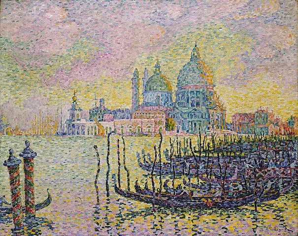
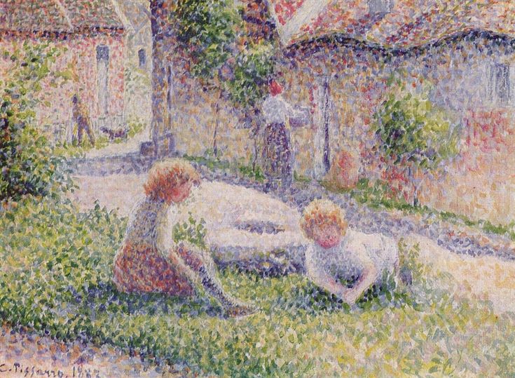
Long before computers, the pointillists had already discovered that a whole scene can be built from thousands of tiny, individually meaningless marks. Seurat and Signac painted with dots of pure color that the eye blends into light and form. Look closely and you see the primitives; step back and you see the picture.

Gaussian Splatting [1: 3D Gaussian Splatting for Real-Time Radiance Field Rendering; Kerbl, Bernhard, Kopanas, Georgios, Leimkühler, Thomas, Drettakis, George; 2023] is the 3D version of the same idea. A scene is represented by millions of small, semi-transparent 3D blobs (Gaussians). Each one carries a position, a shape, a color and an opacity, and when they are blended together from a given viewpoint they reproduce a photograph of the scene. Because the whole representation is differentiable, the blobs can be optimized directly against a set of input images until the rendering matches reality.

Gaussian Splatting is excellent at novel view synthesis — generating photorealistic images from new camera positions — but the cloud of blobs is not a surface. For games, VFX, simulation or 3D printing we usually want a mesh: a connected set of triangles. Extracting one from a splat cloud is the core problem this thesis works on.

A crucial distinction runs through the whole project:

What is Gaussian Splatting?

Each Gaussian is an anisotropic 3D blob defined by a mean $\mu$ (its center) and a covariance matrix $\Sigma$ that controls its size and orientation. To keep the covariance valid during optimization, it is factored into a rotation $R$ and a per-axis scale $S$:

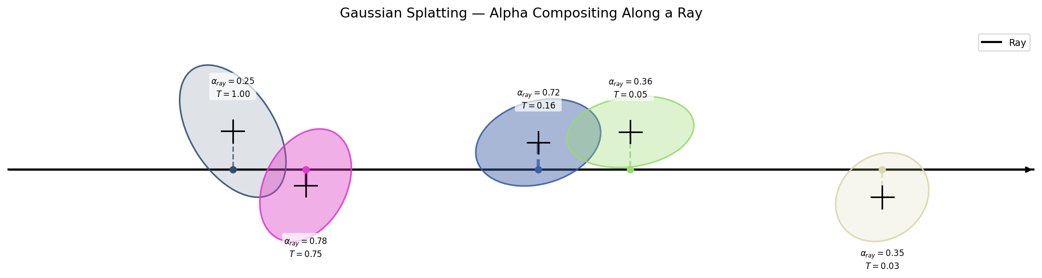
Alongside 1, every splat stores an opacity $\alpha$ and a view-dependent color. To render a pixel, the Gaussians that project onto it are sorted by depth and blended front-to-back with the standard over operator:

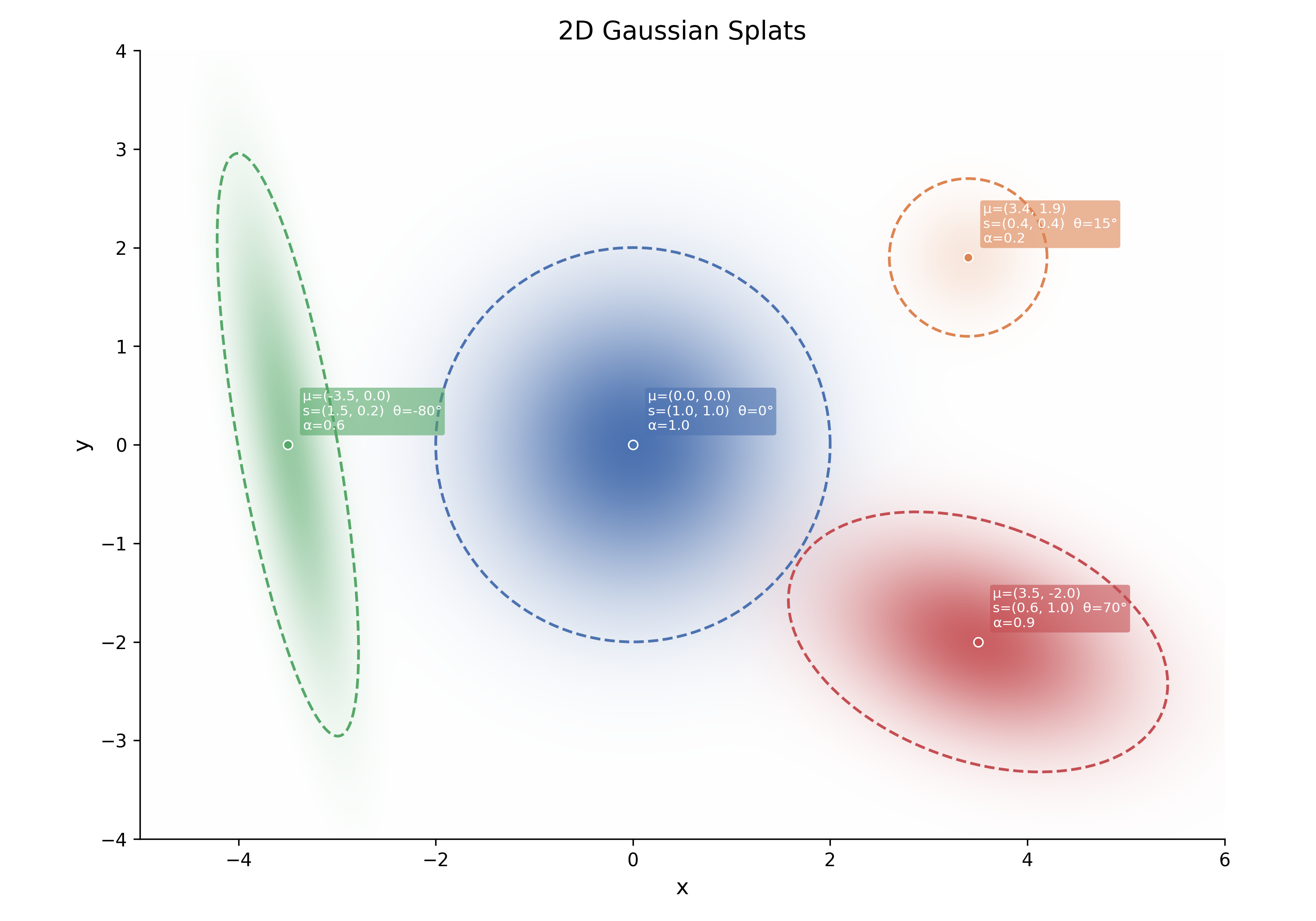
Training is plain gradient descent on the rendered image. The 3DGS loss mixes an $\mathcal{L}_1$ photometric term with a structural (D-SSIM) term:

Two pieces of the pipeline appear repeatedly but are context only for this post — see the Additional context section at the end for detail:

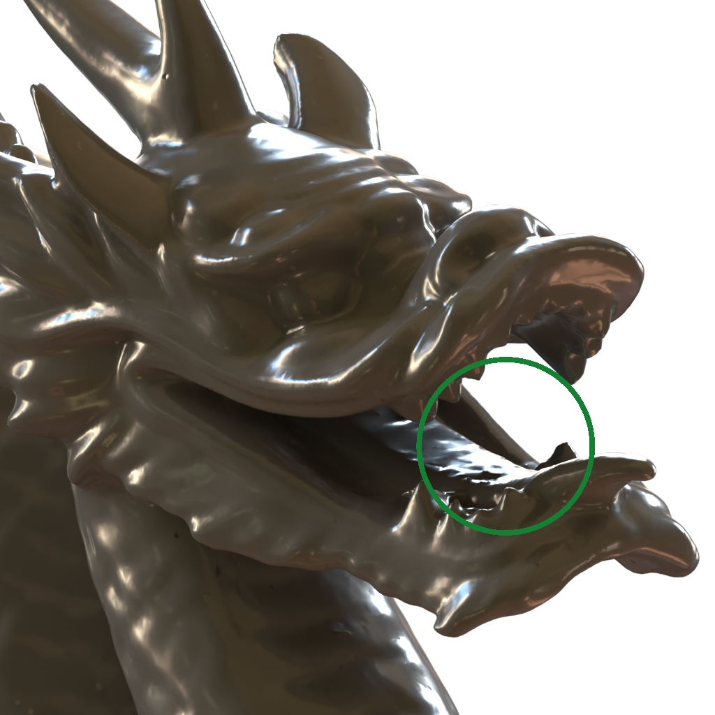
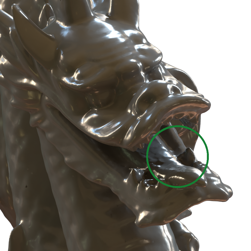
• Spherical harmonics encode the view-dependent color of each splat, so surfaces can change appearance with the viewing angle (specular highlights, Fresnel rim light). See 4 for the effect they capture.
• COLMAP [2: Structure-from-Motion Revisited; Schönberger, Johannes Lutz, Frahm, Jan-Michael; 2016] is the Structure-from-Motion tool that recovers the camera poses and an initial sparse point cloud from the raw photos, before any splatting begins.

From splats to a mesh

To turn the cloud into a surface we need to decide where the surface is. The approach followed here (from GOF [3: Gaussian Opacity Fields: Efficient Adaptive Surface Reconstruction in Unbounded Scenes; Yu, Zehao, Sattler, Torsten, Geiger, Andreas; 2024] and MILo [4: MILo: Mesh-In-the-Loop Gaussian Splatting for Detailed and Efficient Surface Reconstruction; Guédon, Antoine, Gomez, Diego, Maruani, Nissim, Gong, Bingchen, Drettakis, George, Ovsjanikov, Maks; 2025]) attaches geometry to the splats themselves.

Each Gaussian contributes a small set of Delaunay vertices — points placed around its center, offset along its own axes. If $\tilde{s}_k$ is the (inflated) scale of splat $k$ and $b_i$ is a fixed offset direction, vertex $i$ of that splat is:

These vertices are connected by a Delaunay tetrahedralization [5: Computing Dirichlet Tessellations; Bowyer, Adrian; 1981], and each vertex is assigned a signed distance value (inside vs. outside the surface). A differentiable Marching Tetrahedra [6: Deep Marching Tetrahedra: A Hybrid Representation for High-Resolution 3D Shape Synthesis; Shen, Tianchang, Gao, Jun, Yin, Kangxue, Liu, Ming-Yu, Fidler, Sanja; 2021] step then extracts the surface: wherever an edge of a tetrahedron connects an inside vertex $i$ to an outside vertex $j$, a mesh vertex is placed by linear interpolation of their SDF values $f$:

MILo [4: MILo: Mesh-In-the-Loop Gaussian Splatting for Detailed and Efficient Surface Reconstruction; Guédon, Antoine, Gomez, Diego, Maruani, Nissim, Gong, Bingchen, Drettakis, George, Ovsjanikov, Maks; 2025] is the state-of-the-art method that puts this extraction inside the training loop (hence Mesh-In-the-Loop). It makes the per-Gaussian SDF learnable and supervises the extracted mesh directly, comparing the mesh’s own rendered depth $D_M$ and normals $N_M$ against the depth $D$ and normals $N$ of the splat rendering:

Because the mesh is optimized jointly with the splats, MILo produces meshes that are far more faithful than a naive post-hoc extraction.

Contribution 1 — Meshfacto: MILo inside Nerfstudio

MILo’s reference implementation is built on the original 3DGS codebase. My first contribution re-implements its ideas as a first-class method inside Nerfstudio [7: Nerfstudio: A Modular Framework for Neural Radiance Field Development; Tancik, Matthew, Weber, Ethan, Ng, Evonne, Li, Ruilong, Yi, Brent, Wang, Terrance, Kristoffersen, Alexander, Austin, Jake, Salahi, Kamyar, Ahuja, Abhik, Mcallister, David, Kerr, Justin, Kanazawa, Angjoo; 2023], the modular framework whose gsplat [8: gsplat: An Open-source Library for Gaussian Splatting; Ye, Vickie, Li, Ruilong, Kerr, Justin, Turkulainen, Matias, Yi, Brent, Pan, Zhuoyang, Seiskari, Otto, Ye, Jianbo, Hu, Jeffrey, Tancik, Matthew, Kanazawa, Angjoo; 2025] backend is widely used for research. The result is a new method I call Meshfacto, registered as a Nerfstudio entry point and extending its splatfacto model.

Getting there required filling gaps in the stock gsplat backend:

• A median-depth render kernel. gsplat only exposes expected depth; MILo-style supervision needs the more surface-accurate median depth, so a custom backward pass was added.
• A normal render kernel. Surface normals are computed from the depth map with finite differences (depths_to_points → point_to_normal), with a camera-facing sign convention, making the whole normal path differentiable.
• Densification / reinitialization. Instead of relying only on the original adaptive density control, Meshfacto can reinitialize the splats with the depth-based strategy from Mini-Splatting2 [9: Efficient Scene Modeling via Structure-Aware and Region-Prioritized 3D Gaussians (Mini-Splatting2); Fang, Guangchi, Wang, Bing; 2026] [10: Mini-Splatting: Representing Scenes with a Constrained Number of Gaussians; Fang, Guangchi, Wang, Bing; 2024], which redistributes Gaussians onto surfaces far more economically.

Polycount results

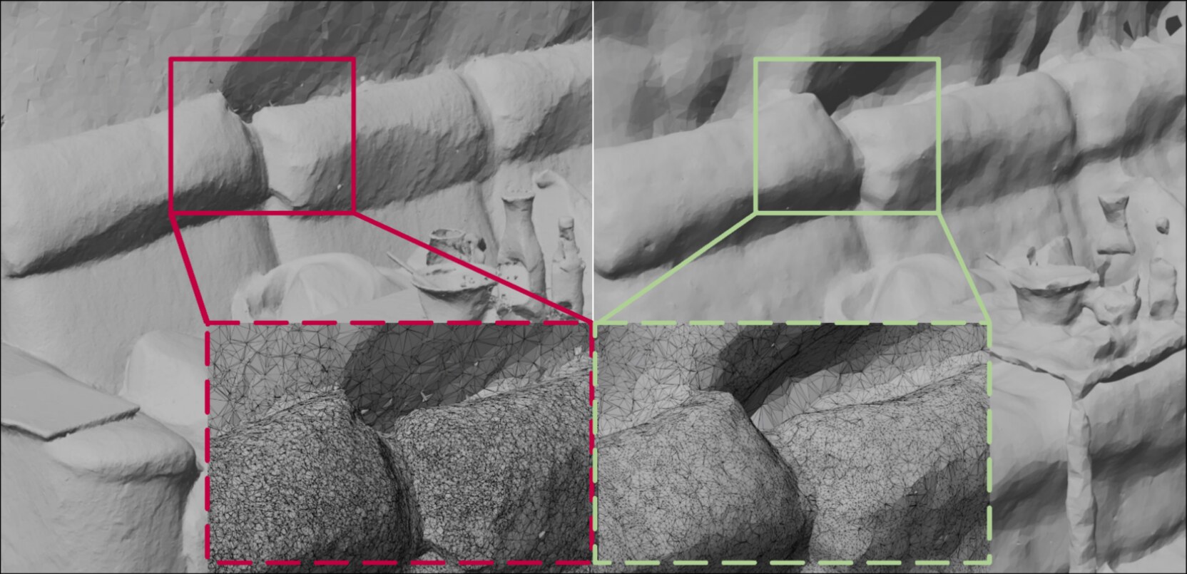
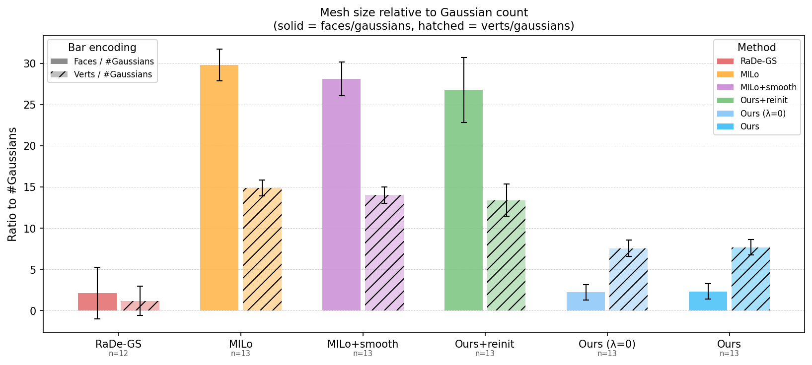
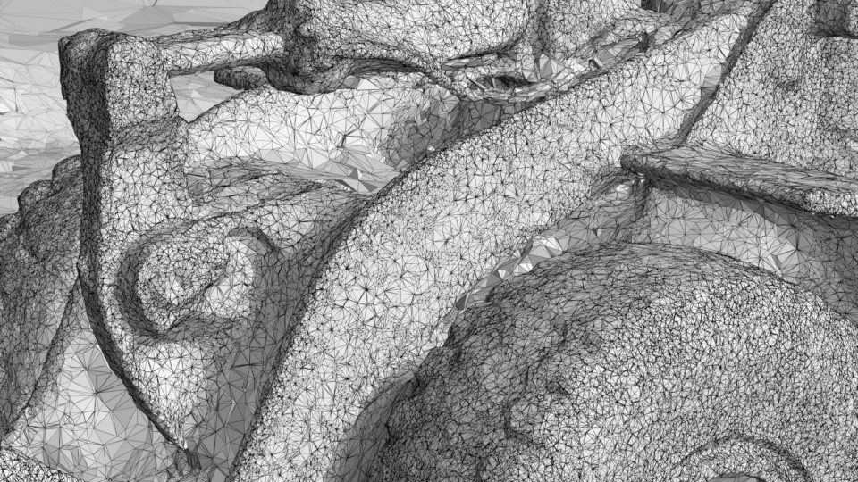
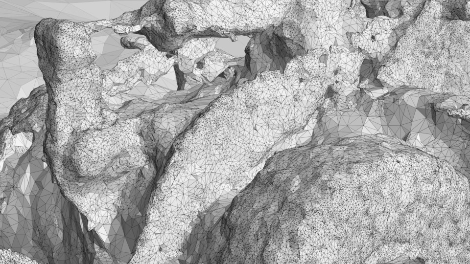
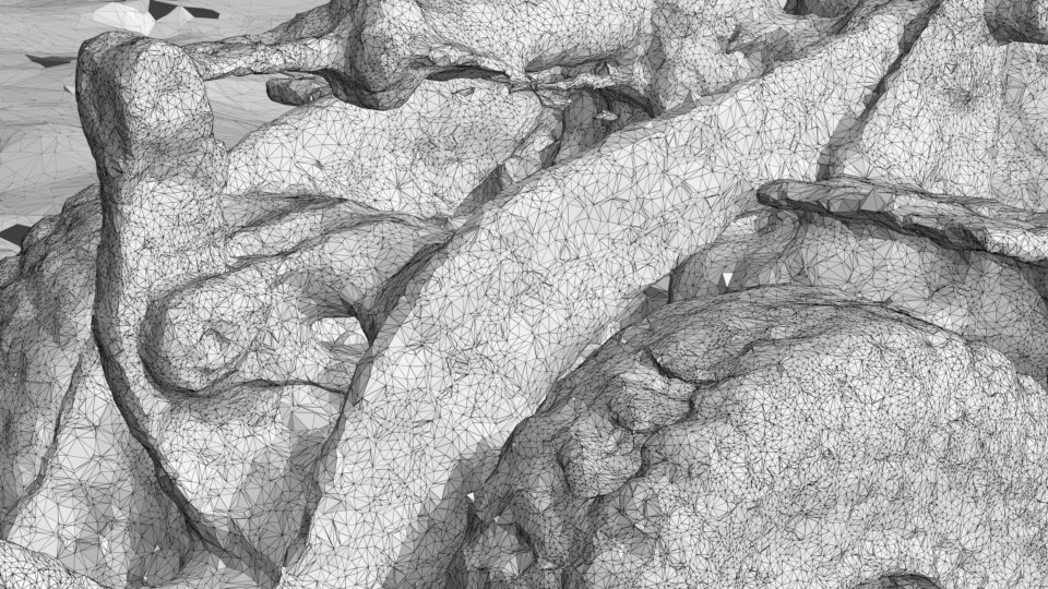
The headline result: at the same Gaussian count, Meshfacto produces meshes with roughly 47% fewer vertices and 76% fewer faces than MILo (base). With Mini-Splatting2 reinitialization enabled (Ours + reinit), the face count drops to about 21–24% of MILo’s while using only a fraction of the Gaussians — on MipNeRF-360, around 0.04M Gaussians versus MILo’s 0.38M.

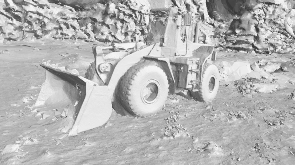
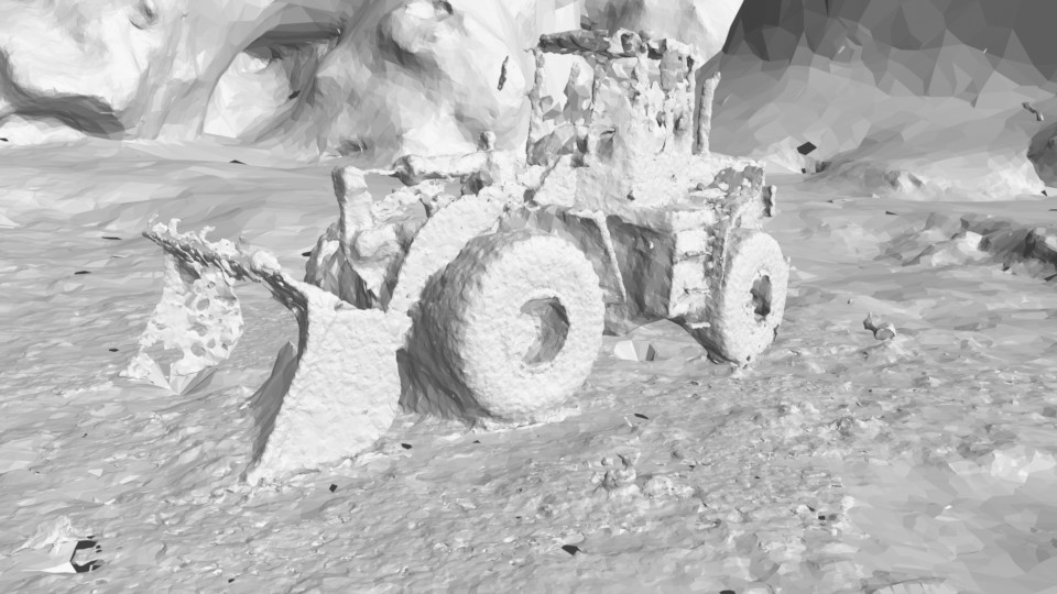
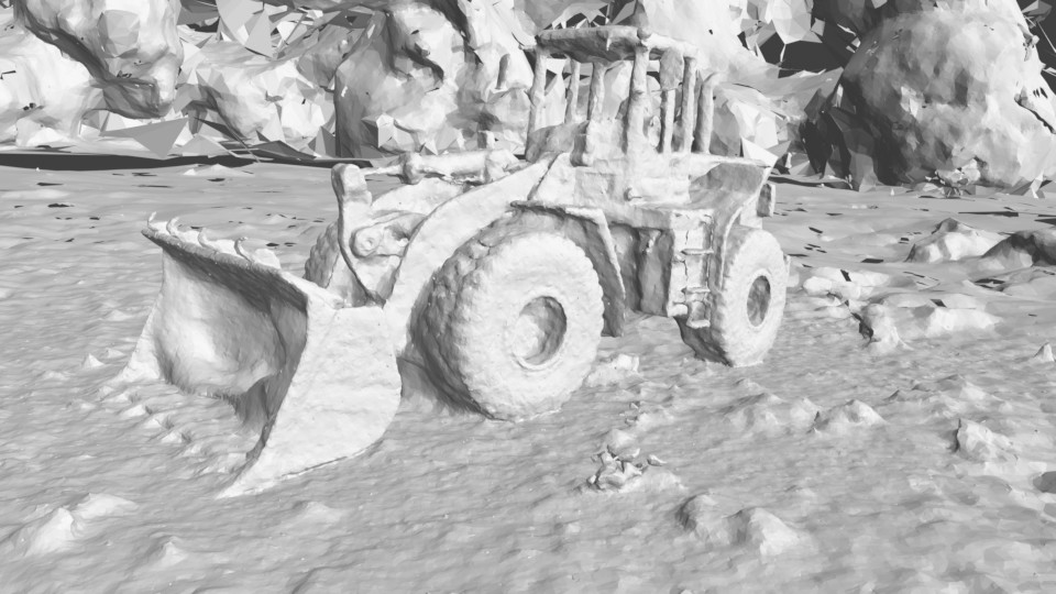
The difference is easiest to see in the wireframes. Below, the same object (the Caterpillar scene from Tanks & Temples [11: Tanks and Temples: Benchmarking Large-Scale Scene Reconstruction; Knapitsch, Arno, Park, Jaesik, Zhou, Qian-Yi, Koltun, Vladlen; 2017]) is reconstructed by MILo, by Ours + reinit and by Meshfacto:

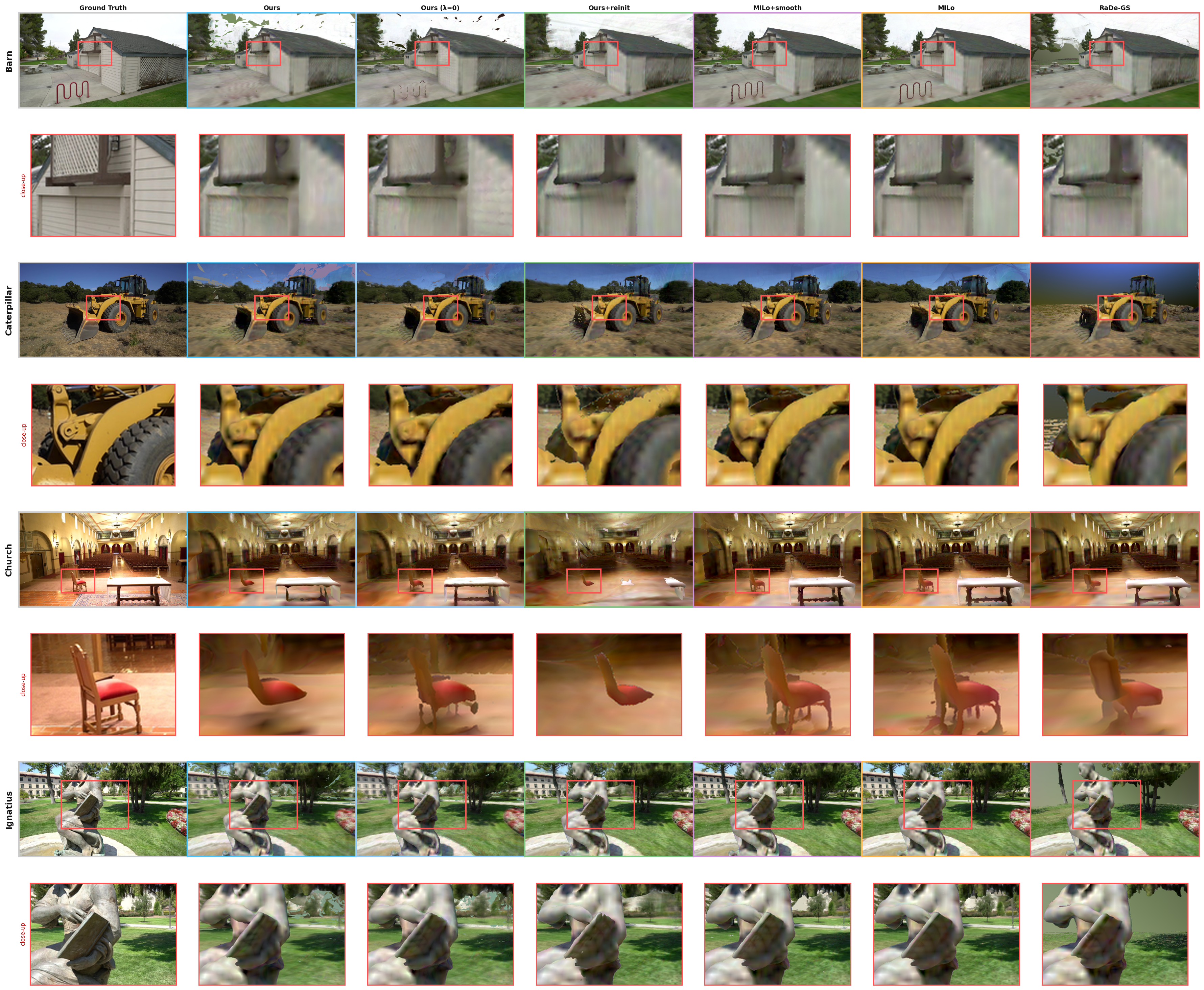
Fewer polygons are only worth it if the surface still looks right. Using MILo’s image-space Mesh-NVS evaluation — rendering novel views from the extracted mesh — the leaner meshes lose only a little quality:

Contribution 2 — Differentiable smoothers

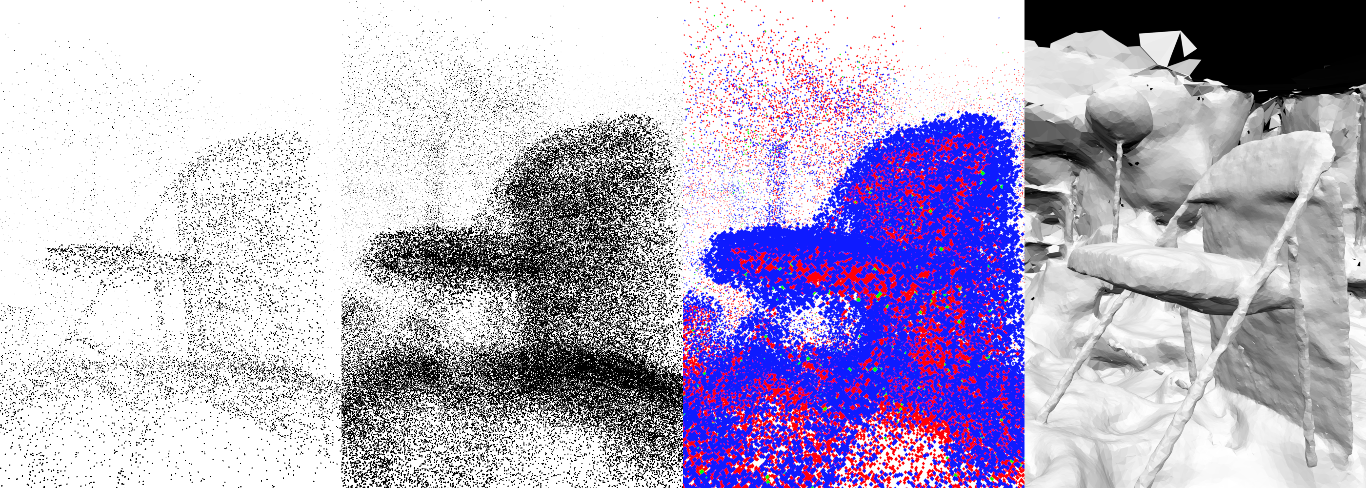
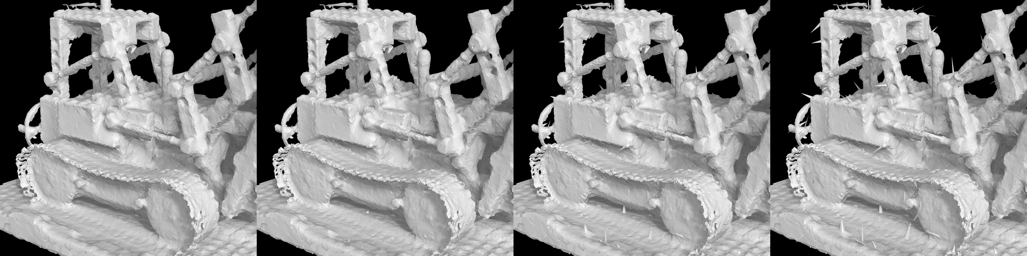
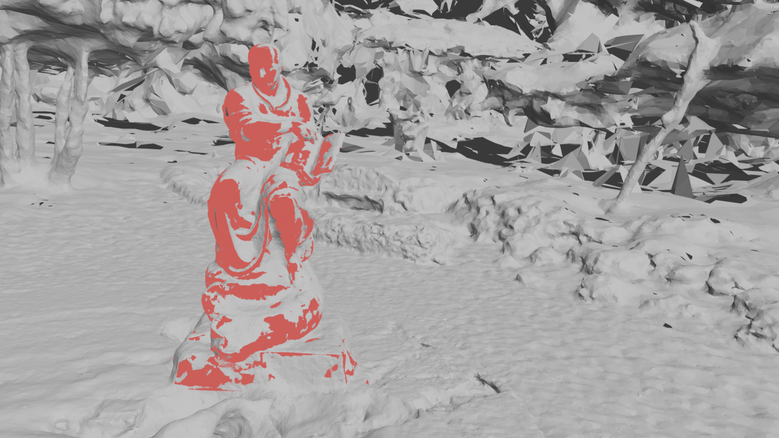
Extracting a mesh inside the training loop has a downside: nothing stops the tetrahedralization from producing degenerate triangles — long, thin slivers that both look bad and destabilize the optimization, since their gradients are ill-conditioned. In early iterations these stretched faces flicker across the surface.

The same problem shows up on real reconstructions. In 12 the degenerate faces are highlighted in red, scattered all over an otherwise clean mesh:

My second contribution adds a family of differentiable smoothing losses that act on the extracted mesh every iteration. Because each mesh vertex depends (through 4 and 5) on the underlying Gaussians’ positions, scales and SDF values, the gradient of these losses flows back into the splats — the mesh gets smoother by nudging the primitives that generate it.

Four losses were studied:

• Uniform (umbrella) Laplacian — pulls each vertex toward the barycenter of its neighbors, encouraging even spacing.
• Cotangent Laplacian — an area-aware variant that respects local curvature.
• Edge-length loss — penalizes the variance of edge lengths, $\mathcal{L}_{\text{edge}} = \mathrm{Var}(\ell_e)$, to curb oversized distant faces.
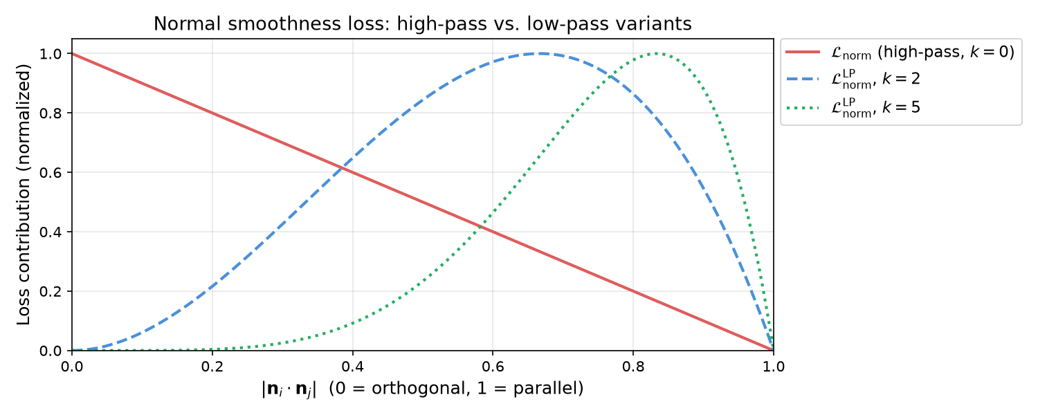
• Normal-smoothness loss — a low-pass filter over face normals, gated by $g_{ij} = |n_i \cdot n_j|^{k}$ so that genuine sharp edges are preserved while noise is smoothed.

The exponent $k$ controls that gate. At $k = 0$ the loss is a high-pass filter that penalizes every normal difference; increasing $k$ turns it into a low-pass filter that ignores near-orthogonal normals (real edges) while still smoothing near-parallel ones:

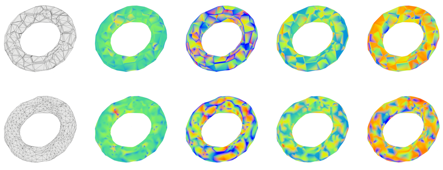
A three-stage sweep (Laplacian-variant selection → per-loss weight → combination) settled on a final recipe: uniform Laplacian ($\lambda = 10$), edge-length loss ($\lambda = 10$), and normal low-pass ($k = 2$). The uniform Laplacian, despite being the simplest, outperformed the area-aware variants here:

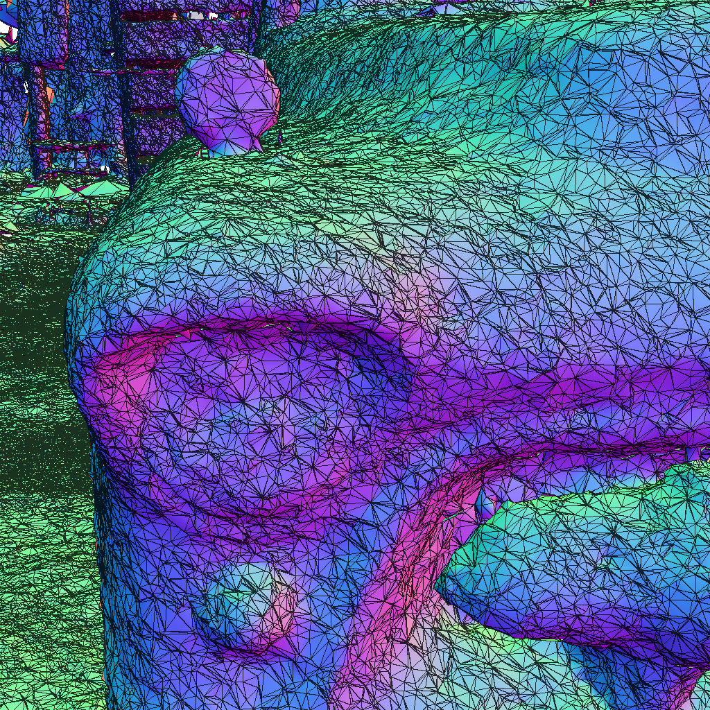
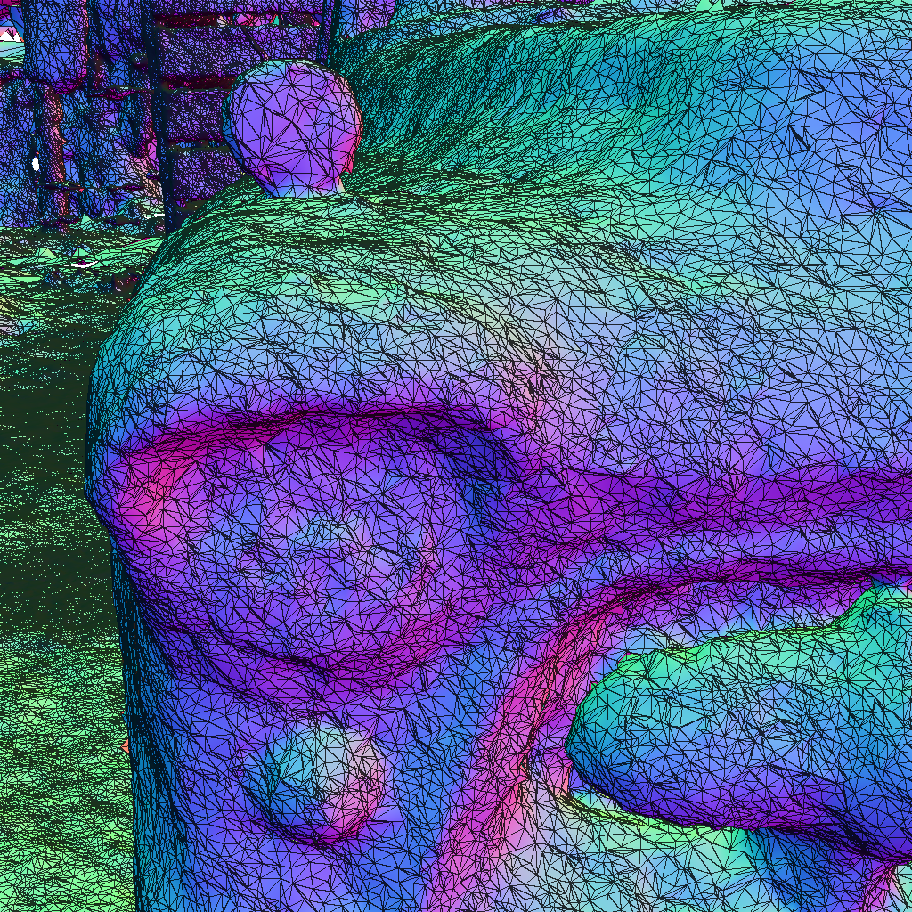
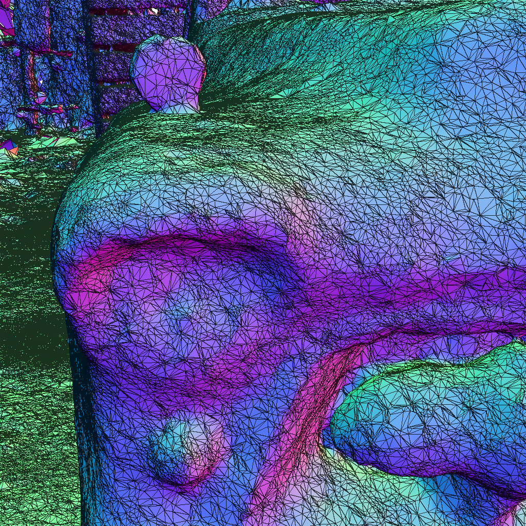
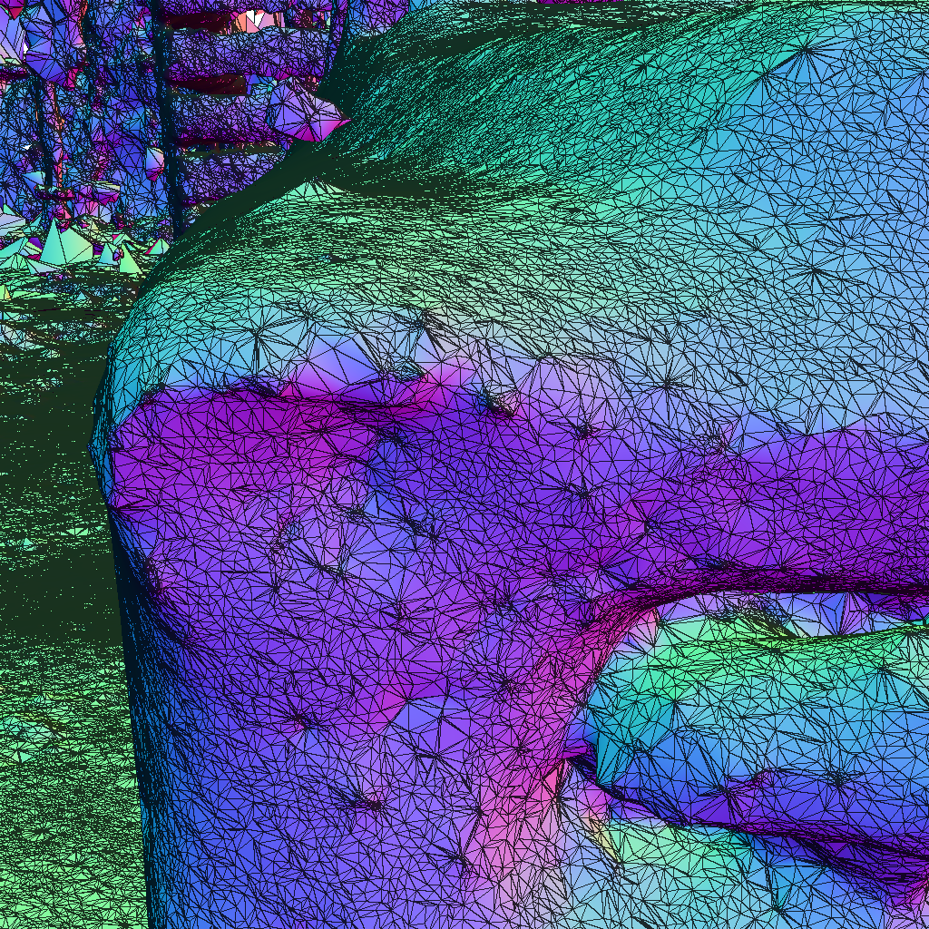
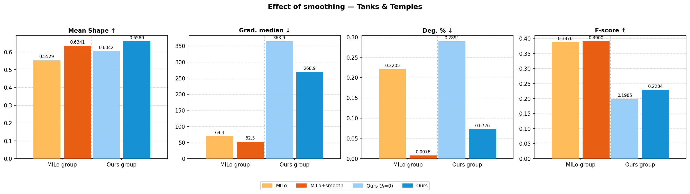
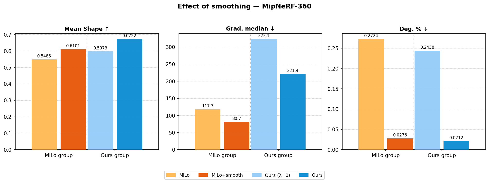
The payoff is measurable. Across Tanks & Temples and MipNeRF-360, the smoothed models improve mesh-quality metrics and, most importantly, drive the fraction of degenerate faces down from about 0.30% to below 0.01% — a ~97% reduction — at a negligible cost in reconstruction fidelity.

Conclusions and future work

Two takeaways stand out. First, the dominant lever for polygon count is the densification / reinitialization strategy — bringing MILo’s mesh-in-the-loop idea into Nerfstudio and pairing it with Mini-Splatting2 reinitialization is what makes the meshes lean. Second, the differentiable smoothers are a conditional but valuable addition: they don’t reduce polygon count on their own, but they regularize the tessellation and stabilize training, nearly eliminating degenerate faces.

Promising directions for future work include geometry-driven densification, decoupling the Delaunay point cloud from the splat cloud, normalizing the smoothing losses by local scale (the coordinate domains of Nerfstudio and COLMAP differ by roughly 5×), and adopting MILo’s TSDF depth-fusion reinitialization.

Additional context

The sections below expand on the background material that the main text kept brief. They are optional reading.

Spherical harmonics

Spherical harmonics [12: Lambertian Reflectance and Linear Subspaces; Basri, Ronen, Jacobs, David; 2001] are an orthonormal basis of functions on the sphere — the angular analogue of a Fourier series. In Gaussian Splatting, each splat stores a small vector of SH coefficients per color channel; evaluating them in the viewing direction gives that splat’s color from the current camera. A degree-3 expansion uses 16 coefficients per channel (48 floats per splat) and is enough to capture soft view-dependent effects such as the specular and Fresnel shading in 4. For pure geometry extraction the SH color is not strictly necessary, but it improves the photometric supervision that drives the whole optimization.

COLMAP and Structure-from-Motion

Before any splatting happens, we need to know where each photo was taken from. Structure-from-Motion (SfM) recovers, from an unordered set of images, both the camera poses and a sparse 3D point cloud. COLMAP [2: Structure-from-Motion Revisited; Schönberger, Johannes Lutz, Frahm, Jan-Michael; 2016] [13: Pixelwise View Selection for Unstructured Multi-View Stereo; Schönberger, Johannes Lutz, Zheng, Enliang, Pollefeys, Marc, Frahm, Jan-Michael; 2016] is the de-facto incremental SfM tool: it detects and matches feature points across images, estimates relative camera geometry, and triangulates 3D points, refining everything with bundle adjustment. Global alternatives such as GLOMAP [14: Global Structure-from-Motion Revisited (GLOMAP); Pan, Linfei, Baráth, Dániel, Pollefeys, Marc, Schönberger, Johannes L.; 2024] trade some robustness for large speedups. The sparse COLMAP point cloud is what initializes the Gaussian splat positions.

Marching Cubes and Marching Tetrahedra

Marching Cubes [15: Marching Cubes: A High Resolution 3D Surface Construction Algorithm; Lorensen, William E., Cline, Harvey E.; 1987] is the classic algorithm for extracting a surface (isosurface) from a scalar field sampled on a regular grid: for each cell it looks up a triangulation from a case table based on which corners are inside vs. outside the surface.

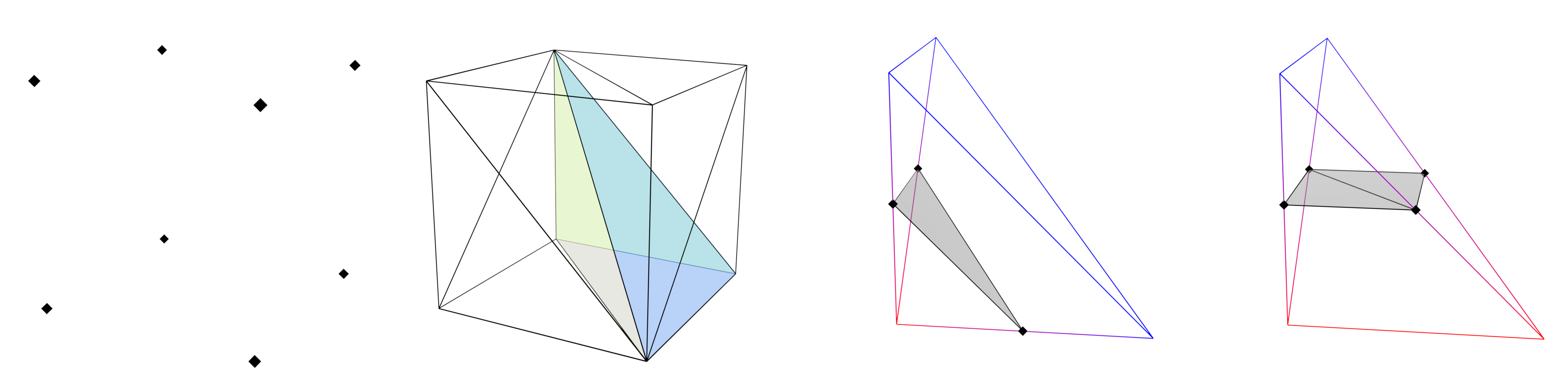
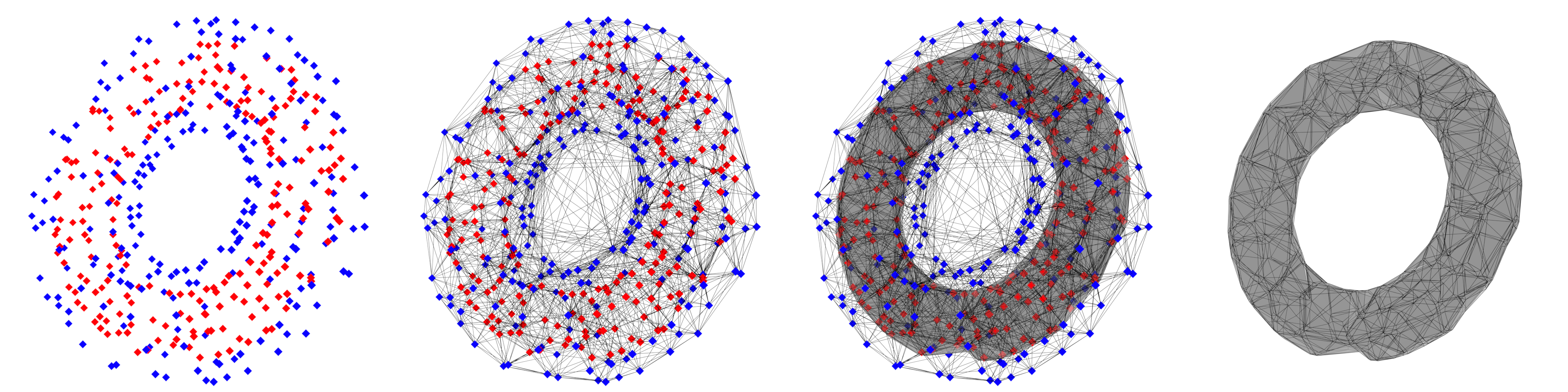
Marching Tetrahedra is the tetrahedral counterpart. It is attractive here because the cell structure can follow an irregular, scene-adaptive Delaunay tetrahedralization rather than a fixed grid, and — crucially — its interpolation step (5) is differentiable, so gradients from the mesh flow back to the field values.

Mesh-quality metrics

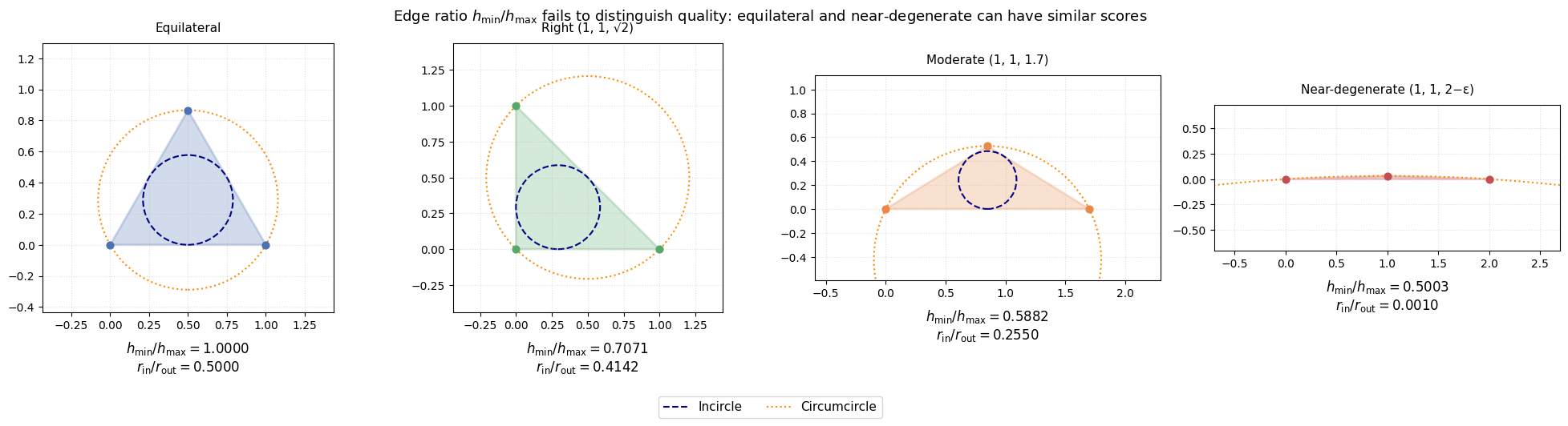
To evaluate tessellation quality objectively, the thesis uses local shape metrics such as the mean-ratio $S_3$ (how close a triangle or tetrahedron is to equilateral), the fraction of degenerate faces, and a global gradation metric measuring how smoothly element sizes vary across the mesh. Two triangles can share the same edge-length ratio yet differ wildly in angles — 18 illustrates why a single ratio is not enough and multiple indicators are needed.

Sustainability and licensing

All experiments ran on a single consumer GPU (RTX 5070, 12 GB), with each full run taking roughly 40 minutes to 2 hours — a fraction of the compute assumed by the reference MILo setup (RTX 4090, 24 GB). On the legal side, the Meshfacto core stays compatible with permissive licenses: Nerfstudio and gsplat are Apache-2.0 [16: Apache License, Version 2.0; Apache Software Foundation; 2004], while some upstream components (MILo’s Gaussian-Splatting License [17: Gaussian-Splatting License; Inria, Max Planck Institute for Informatics; 2023] and nvdiffrast’s NVIDIA source license [18: NVIDIA Source Code License (1-Way Commercial); NVIDIA Corporation; 2020] [19: Modular Primitives for High-Performance Differentiable Rendering (nvdiffrast); Laine, Samuli, Hellsten, Janne, Karras, Tero, Seol, Yeongho, Lehtinen, Jaakko, Aila, Timo; 2020]) are non-commercial — worth keeping in mind for any downstream use.

Bibliography

- , "3D Gaussian Splatting for Real-Time Radiance Field Rendering", ACM Transactions on Graphics, vol. 42, 2023, DOI | URL.
- , "Structure-from-Motion Revisited", 2016.
- , "Gaussian Opacity Fields: Efficient Adaptive Surface Reconstruction in Unbounded Scenes", ACM Transactions on Graphics, vol. 43, 2024, DOI.
- , "MILo: Mesh-In-the-Loop Gaussian Splatting for Detailed and Efficient Surface Reconstruction", ACM Transactions on Graphics, 2025, URL.
- , "Computing Dirichlet Tessellations", The Computer Journal, vol. 24, pp. 162–166, 1981, DOI.
- , "Deep Marching Tetrahedra: A Hybrid Representation for High-Resolution 3D Shape Synthesis", 2021.
- , "Nerfstudio: A Modular Framework for Neural Radiance Field Development", 2023, DOI.
- , "gsplat: An Open-source Library for Gaussian Splatting", Journal of Machine Learning Research, vol. 26, pp. 1–17, 2025.
- , "Efficient Scene Modeling via Structure-Aware and Region-Prioritized 3D Gaussians (Mini-Splatting2)", IEEE Transactions on Pattern Analysis and Machine Intelligence, vol. 48, pp. 4623–4641, 2026, DOI.
- , "Mini-Splatting: Representing Scenes with a Constrained Number of Gaussians", 2024, DOI.
- , "Tanks and Temples: Benchmarking Large-Scale Scene Reconstruction", ACM Transactions on Graphics, vol. 36, 2017, DOI.
- , "Lambertian Reflectance and Linear Subspaces", 2001, DOI.
- , "Pixelwise View Selection for Unstructured Multi-View Stereo", 2016.
- , "Global Structure-from-Motion Revisited (GLOMAP)", 2024, DOI.
- , "Marching Cubes: A High Resolution 3D Surface Construction Algorithm", SIGGRAPH Computer Graphics, vol. 21, pp. 163–169, 1987, DOI.
- , "Apache License, Version 2.0", 2004, URL.
- , "Gaussian-Splatting License", 2023, URL.
- , "NVIDIA Source Code License (1-Way Commercial)", 2020, URL.
- , "Modular Primitives for High-Performance Differentiable Rendering (nvdiffrast)", ACM Transactions on Graphics, vol. 39, 2020.