Color Management for Multimedia Applications
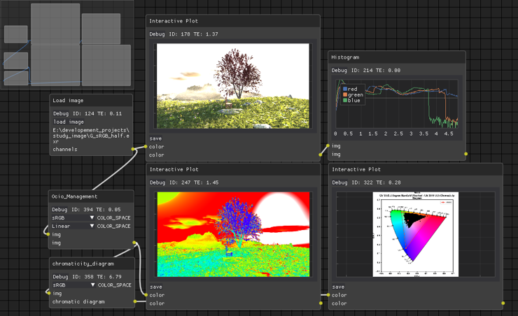
This is the digital version of my bachelor’s thesis, Development of an Application for Color Management in Multimedia Environments. It is a complete, from-scratch introduction to digital color science — how light becomes a photograph, how a photograph becomes a file, and how that file ends up looking right (or wrong) on a screen — paired with Study Image, a node-based Python application I built so every one of those steps can be seen and tested instead of taken on faith.
- Motivation
- Digital color science
- Display technology
- A proposed open color pipeline
- Study Image: a node-based tool for studying color
- A Blender color-management addon
- Conclusion
- Bibliography
Motivation
Free material on color science tends to be scattered and incomplete: a post explains gamma, another explains gamuts, a third explains RAW processing, and none of them connect into a full picture of what happens to an image between capture and display. Having worked as a VFX, compositing and color-grading supervisor on several university productions, I kept running into the same gap — artists and generalists picking up half-explained terminology and, as a result, misconfiguring color pipelines in ways that are hard to diagnose later.
This thesis tries to close that gap with two things: a complete, ordered explanation of color management aimed at artists rather than engineers, and a piece of software, Study Image, that lets you see the concepts — color space primaries, transfer functions, dynamic range, file formats — instead of taking them on faith.
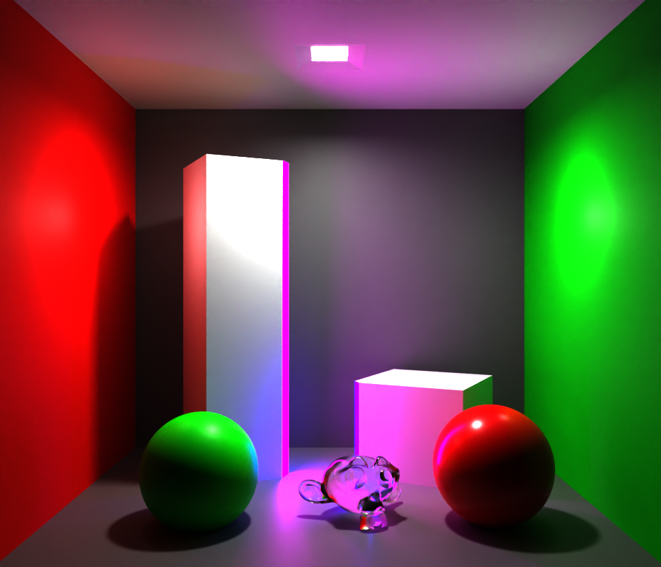
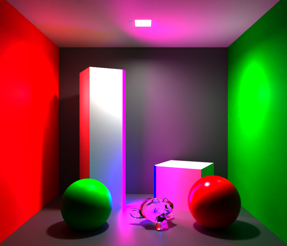
A recurring theme throughout: the render color space itself changes the final image, independently of any later color-space conversion. Two scenes lit with identical sRGB-defined colors but rendered internally in sRGB vs. ACEScg do not converge to the same result after converting both back to sRGB — the highlights saturate and roll off differently. This is one of the most under-documented behaviors in day-to-day CG color work, and a large part of the thesis is spent making it legible.
Digital color science
Digital color science is the study of how colors are created, measured, captured, reproduced and perceived across digital systems [1: The Principles of Color Management; 2009] — a field that spans far more than “color management” alone: from the physics of light, through sensors and renderers, to file formats and the screens that finally display them.
The current paradigm
Digital color science is extensive and spans many disciplines, and it developed very quickly, chasing hardware that itself kept evolving. That history left behind a wide, inconsistent nomenclature that is a real barrier for newcomers.
A small example makes this concrete. Mobile screens, computer monitors and televisions can often all emit the same set of colors, called sRGB — yet the same content still looks different across them. That’s because of the transfer function layered on top of the primaries: TVs typically use a curve called rec.709, while computer and phone screens use a curve called sRGB (confusingly, the same name as the color space). To complicate things further, there are two curves both called “sRGB”: one is an exact piecewise formula, the other an approximation often written “~gamma 2.2” that differs mainly in the shadows. A color space is defined by more than just its range of colors, and every one of those extra properties matters for correct color management — this thesis works through them one at a time.
Scene-Referred vs. Display-Referred
Two concepts run through the whole pipeline:
- Scene-Referred — values that represent the linear light of a real (or simulated) scene, exactly as captured.
- Display-Referred — values that have been reshaped, usually with a perceptual/logarithmic curve, to be shown on a screen, the same way our own eyes compress the light they receive.

The basics of light
To understand dynamic range and primaries, it helps to start from the actual physical behavior of light. The units that matter across a digital image’s lifetime:
- Photons — light itself, and its frequency (color). Sensors receive photons directly.
- Candela — the SI base unit of luminous intensity.
- Nits — one nit equals one candela per square meter; used for the light emitted by screens. Ordinary displays run around 100 nits, HDR displays at 1000–10000 nits.
- Watts — the unit 3D renderers and ray tracers actually compute in (0.05 W ≈ 1 candle). As reference points [2: Light Objects; 2023]: a clear sky ≈ 1000 W/m², an overcast sky ≈ 500 W/m², a very overcast sky ≈ 200 W/m², a full-moon night ≈ 0.001 W/m².
From real color to digital color
Light is rarely a single wavelength (510 nm for green, say) — it’s a spectrum, many frequencies combined, and the surfaces it bounces off reflect a new, altered spectrum [3: Artificial Lighting System for Plant Growth and Development: Chronological Advancement, Working Principles, and Comparative Assessment; ; 2017]. The color of the light source itself has a direct effect on perceived color too: a UV blacklight is the extreme case, making some pigments fluoresce brightly while leaving others completely unaffected.
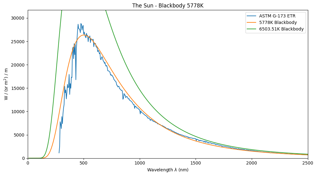
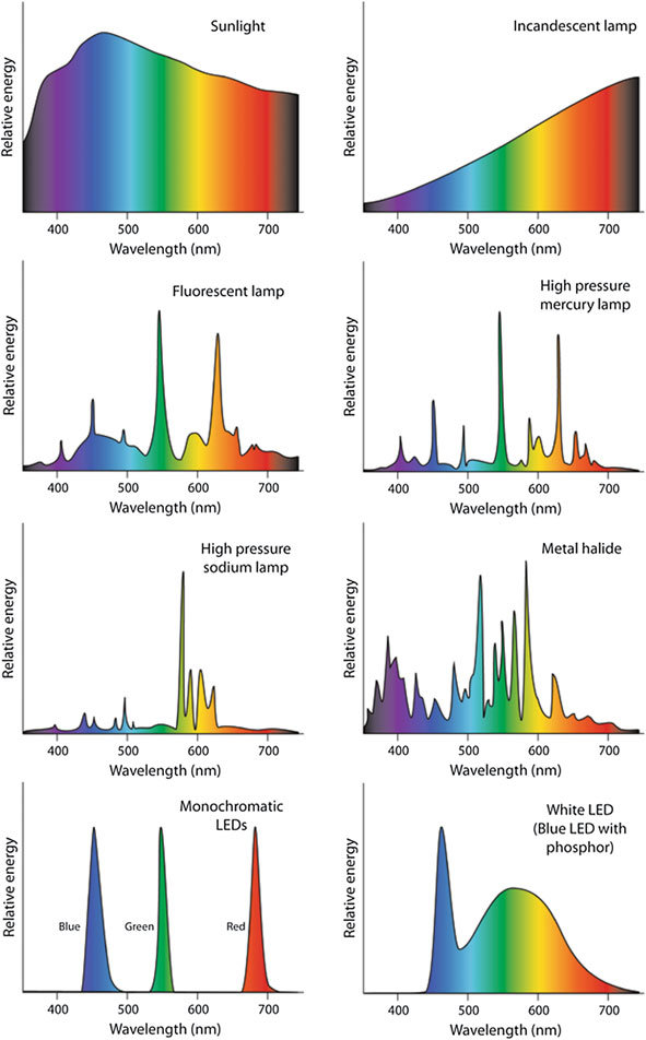
To go from a real spectrum to something representable digitally, we lean on metamerism: the phenomenon where two color samples match under one set of viewing conditions (light source, observer, geometry) but not under another. Converting a spectrum into RGB means finding a new spectrum — one a screen’s monochromatic LEDs can actually emit — that produces the same visual response.
Working from the premise that any color can be described as a mix of three primaries, the CIE defined the CIE XYZ color space [4: Colorimetry - 4th Edition; ; 2018], built from human cone-response experiments (William David Wright and John Guild measured how sensitive human eyes are to monochromatic light at different wavelengths) so that it contains every color a human eye can see. Each XYZ value runs 0–100; Y carries luminance, X is roughly “red vs. green” energy, and Z is roughly “blue vs. yellow” energy.
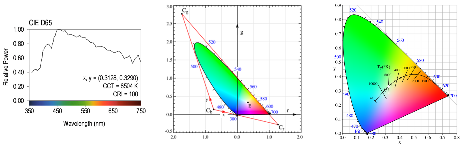
XYZ is turned into the familiar 2D chromaticity coordinates xy (dropping luminance) simply by normalizing:
Converting XYZ into an RGB working space should look perceptually similar no matter which space you land in. 4 shows the same real color-checker patches: their real xy positions on the left, then re-plotted inside sRGB and ACEScg. In sRGB the patches crowd toward the center — the space physically cannot hold their real saturation — while in ACEScg they land almost exactly where their real coordinates say they should.
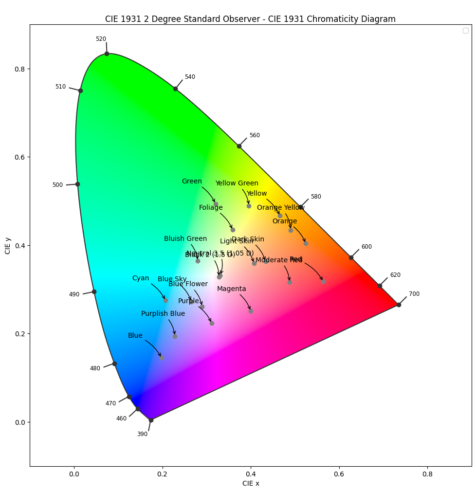
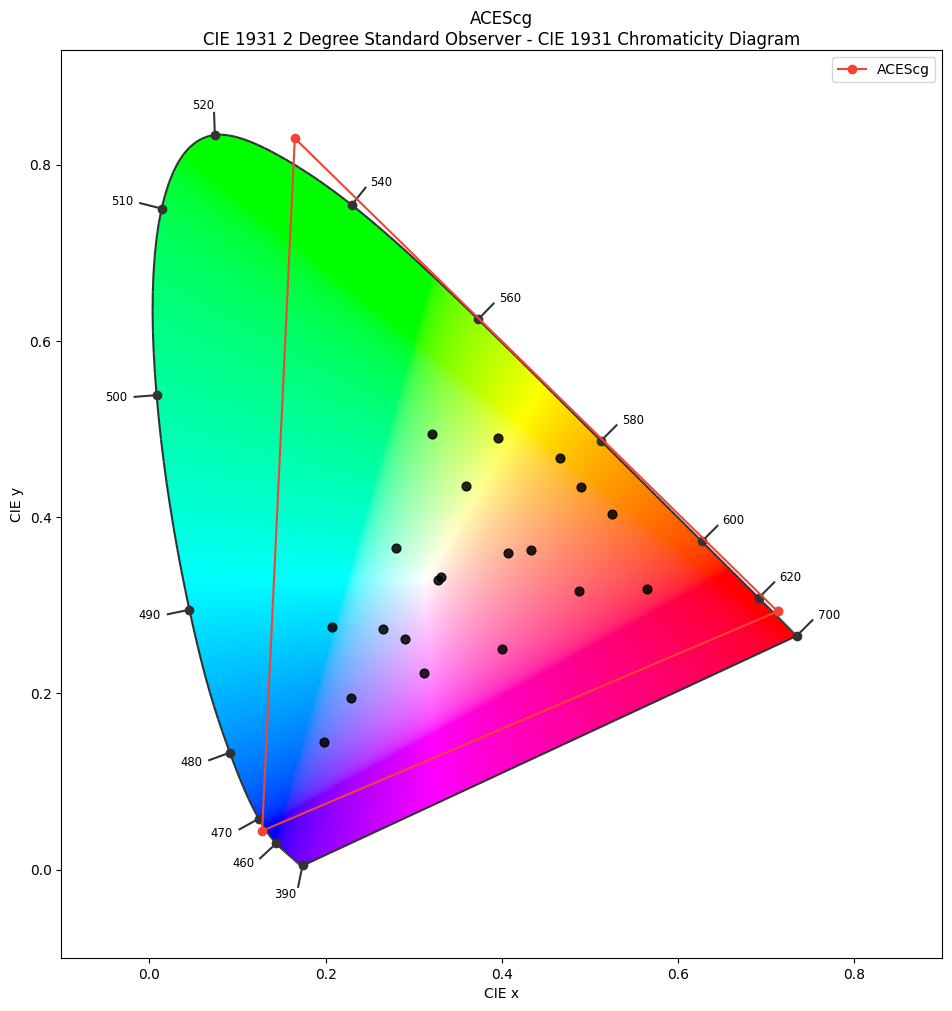
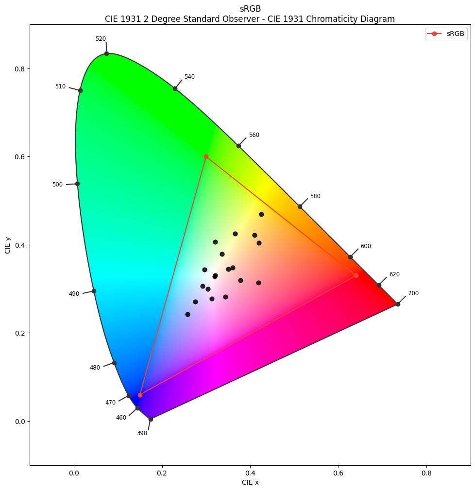
This is why a sRGB screen, which can’t reproduce every color, can still show a difference between two colors that are both technically outside its gamut — a green patch will look less saturated on an sRGB screen than on an ACEScg one (no screen can actually show the full ACES gamut, but the point stands for wide-gamut displays). Matching a real, known color across multiple devices is genuinely hard, and artistic decisions inevitably creep in to make the result “look more believable.”
RAW: a worked example of the full pipeline
RAW processing is a clean, concrete example of the whole color pipeline in miniature. In an analog camera, exposure blackens a photosensitive film; a digital camera replaces the film with a sensor made of pixels, each storing how many photons it received during the exposure. The sensor’s dynamic range is limited by how many photons it can register at minimum and maximum, and by pixel noise and saturation — the camera (or the photographer) has to choose which slice of the light to keep.
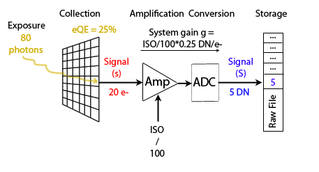
RAW formats vary by manufacturer (Nikon NEF, Canon CR2, Sony SR2, Pentax PTX, Olympus ORF, Fujifilm RAF, Panasonic RAW2…), but they all store the same kind of thing: a 2D matrix in Bayer pattern, one color per photosite, Scene-Referred. Getting from that matrix to a finished image follows a fixed sequence of steps:
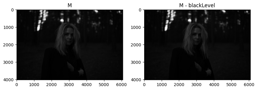
1. Black-level subtraction. Even with zero light, a sensor’s pixels register a small baseline signal specific to the camera hardware, which must be subtracted per channel before anything else.
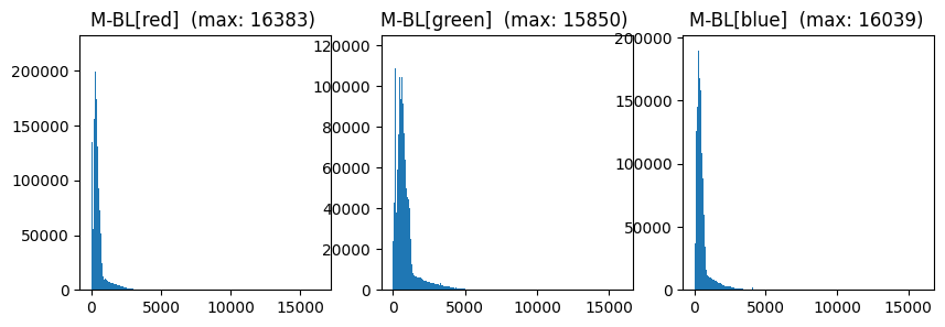
2. White balance. A per-channel multiplier that makes a chosen reference read as pure white, correcting for the scene’s illuminant — this is usually stored right in the RAW file’s metadata (e.g. [1.74, 1, 1.58, 1] for [R, G, B, G]).
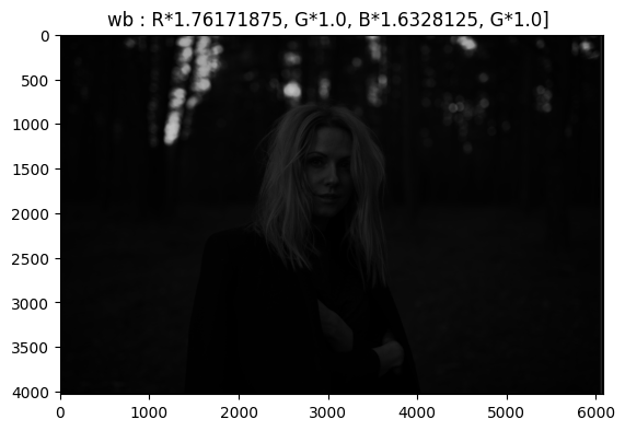
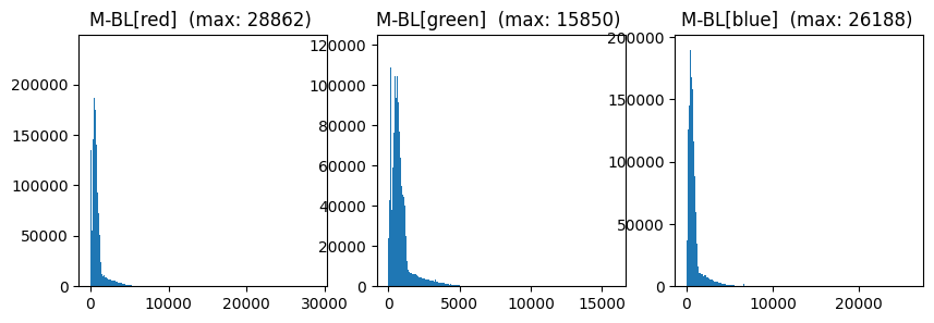
3. Correct the light level (only relevant in fixed-precision formats). A photographed scene’s linear light typically spans about 14 EV, encoded in 14 bits. Editing that in a 16-bit-integer environment without rescaling makes the image look about 4× darker than it should — the fix is to redistribute those 14 bits of range across the full 16-bit container. (Working in float32, as most editing software does, avoids this problem entirely, since the image is normalized against its own maximum value.)
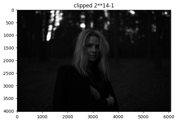
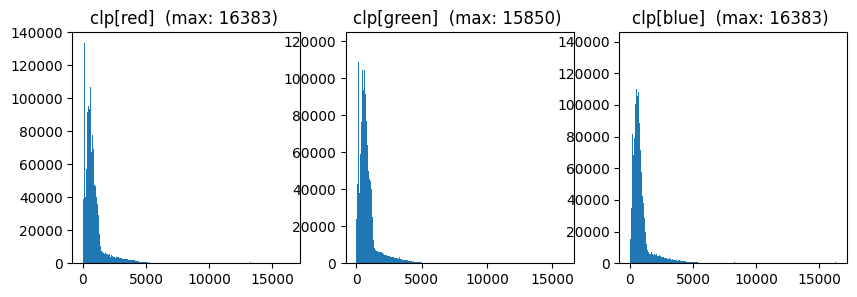
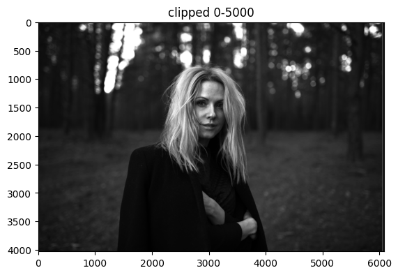
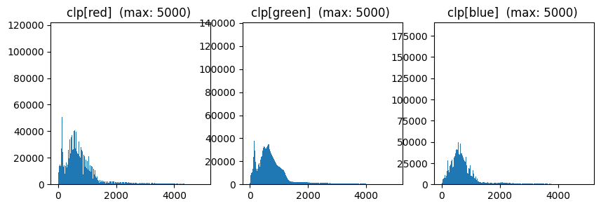
4. Highlight reconstruction. After white balance, the red and blue channels usually clip above the green channel’s own maximum — normalizing again produces an ugly cast, since green loses information the other two channels still have.
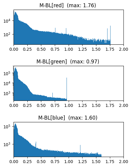
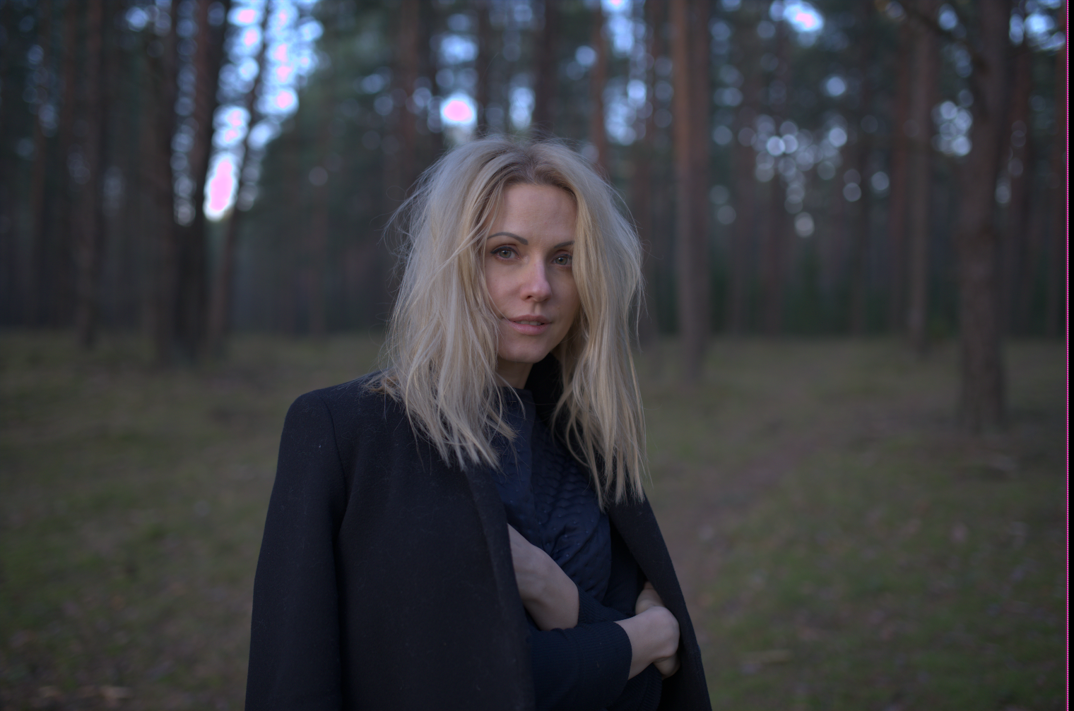
The simplest fix, clip, just discards the overflow and loses roughly 2/3 of an EV of highlight detail. A better one, mean, recovers that lost range by averaging the red and blue channels back into blown-out green pixels:
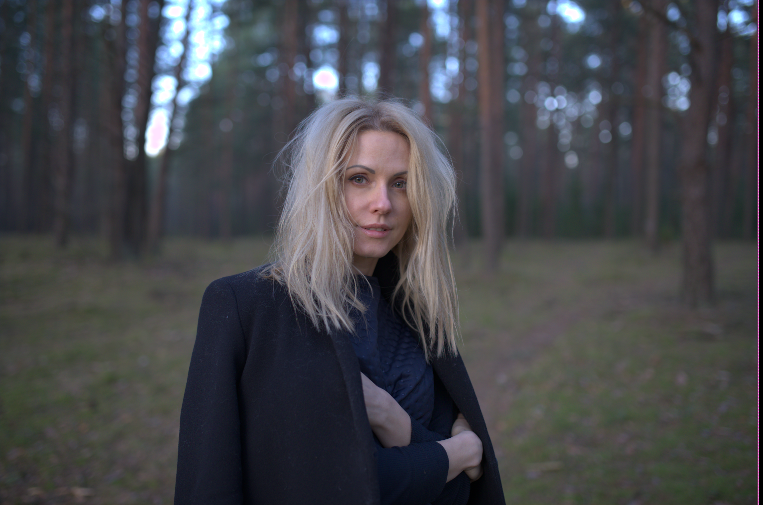
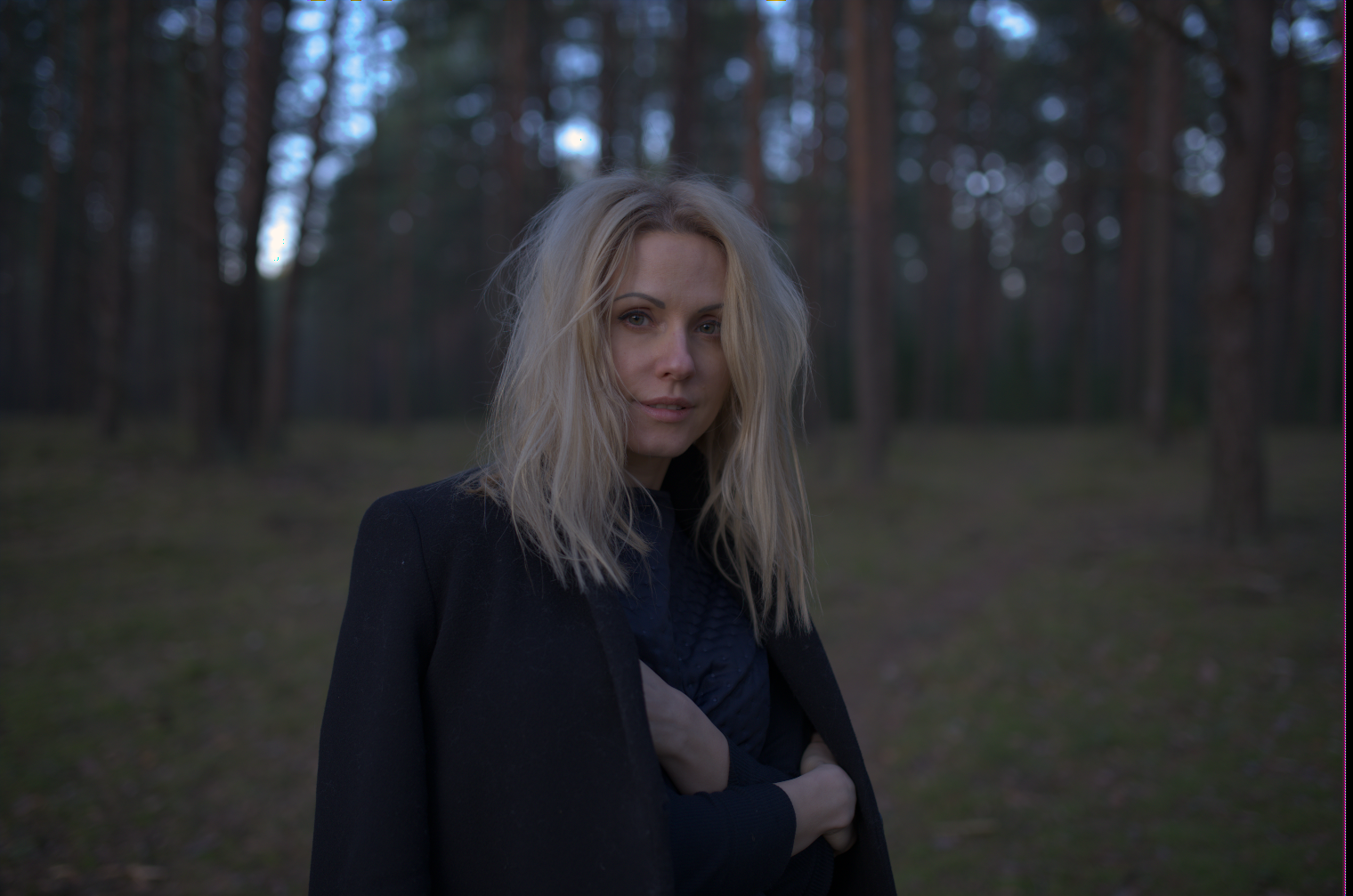
More elaborate reconstruction methods exist too — reconstructing in LCh space from unclipped neighboring pixels, transferring color information from unclipped regions, or guided-Laplacian gradient propagation, all used by tools like darktable.
5. Demosaicing. The sensor is covered by a color filter that only lets specific wavelengths reach specific photosites — each pixel only ever records one channel natively. Demosaicing interpolates the missing two channels from neighboring pixels. The simplest scheme, bilinear, just averages same-channel neighbors:
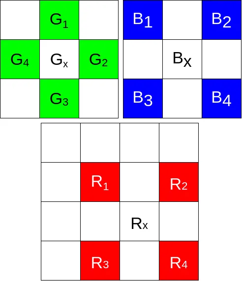
(More sophisticated schemes — Malvar2004, Menon2007, DDFAPD — do better by adapting to local edges and gradients instead of blindly averaging.)
6. Color transformation and correction. The sensor’s RGB response doesn’t match human perception, so the camera manufacturer photographs known color-checker patches and derives a 3×3 matrix that maps the camera’s native RGB into CIE XYZ. That matrix ships in the RAW file’s metadata.
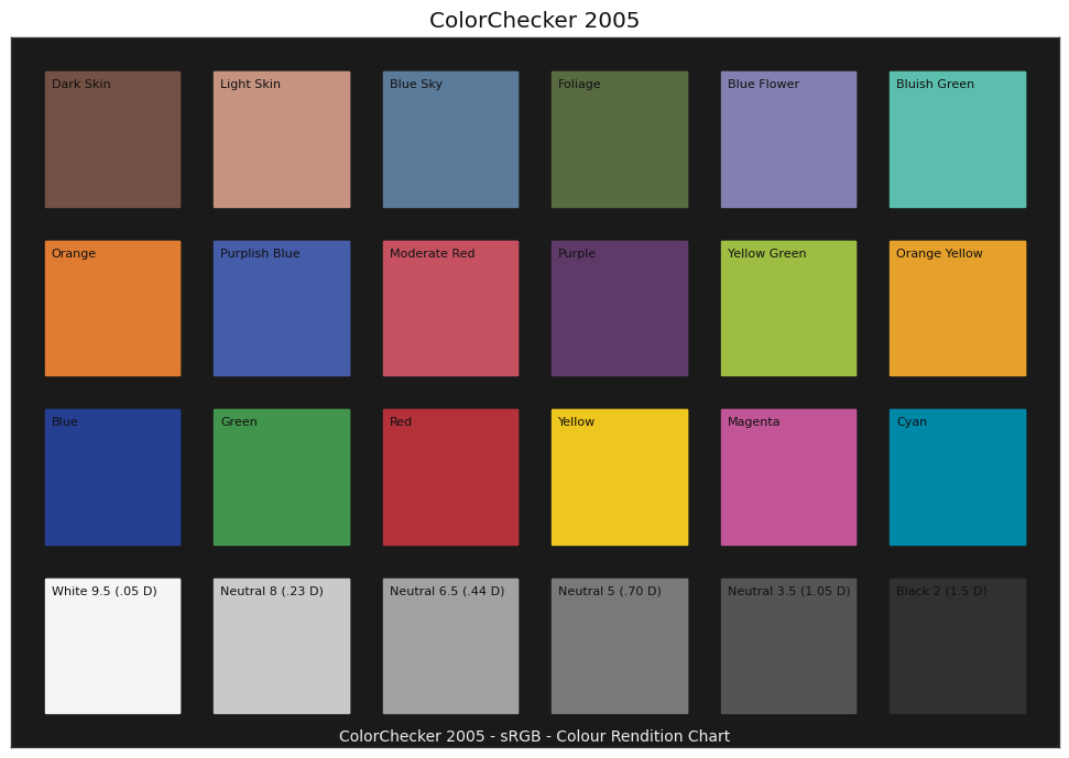
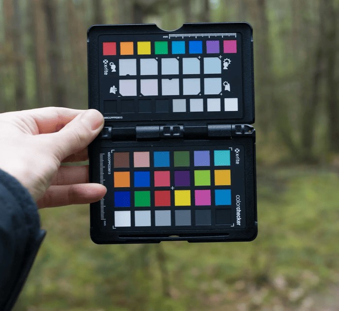
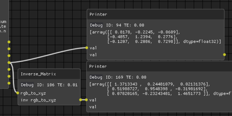
That raw matrix has one problem: a pure white input (R=G=B=1) needs to produce luminance Y=1, and it doesn’t out of the box — so it gets renormalized against a chosen white-point illuminant (D65 for daylight, D50 for print viewing conditions, etc.) before use.
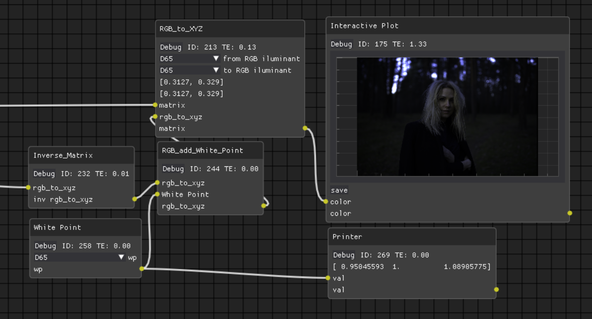
Once the data sits in a standardized space, it can go anywhere — here, sRGB under both D65 and D50:
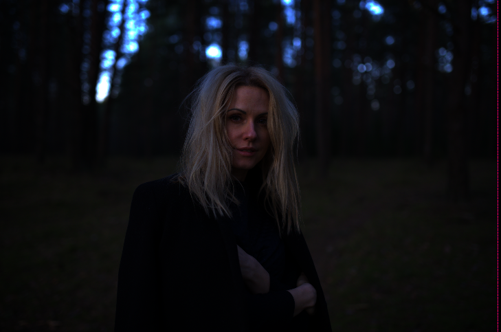
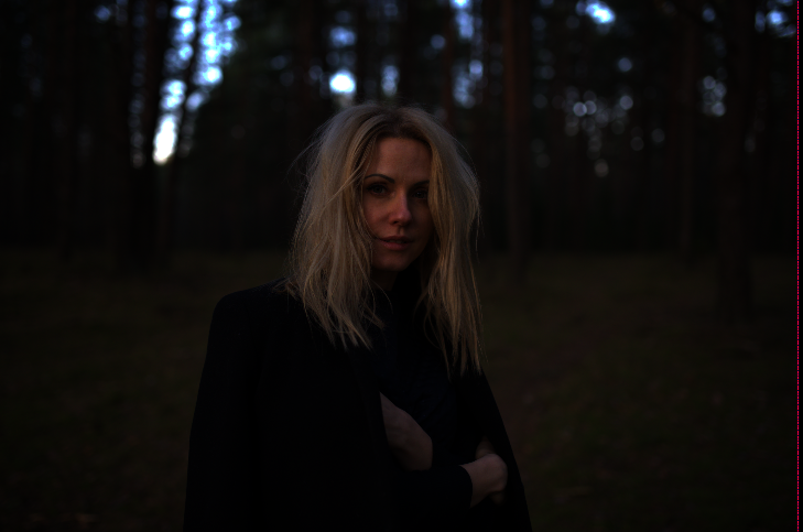
7. Apply the transfer function (OETF). Only at the very end does a curve like the sRGB OETF get applied — the sRGB space uses gamma = pixel^(1/2.2) going out to a display, and a display itself applies gamma = pixel^2.2 to invert it.
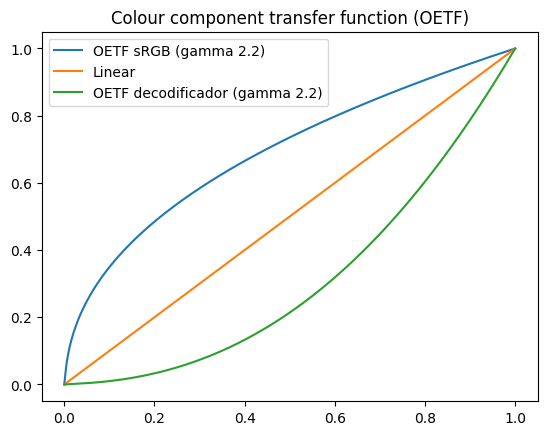
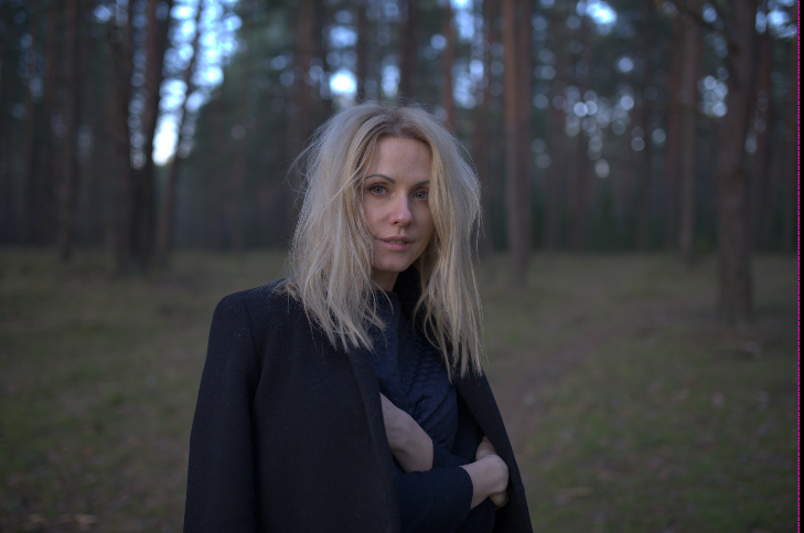
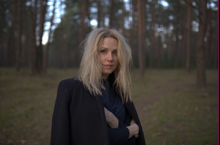
A gamma function is a pure exponential; an OETF is a more elaborate curve that doesn’t have to follow a strict exponent, often written with a tilde (~gamma 2.2) to signal “close to, but not exactly.” Applying the sRGB OETF is what turns the darker-looking linear renders above into a finished, displayable photograph:
Why CGI isn’t RAW
Computer-generated images work differently. There’s no real light to demosaic — a renderer’s “virtual sensor” is assumed lossless, printing exactly what the simulation computes, so final image quality is a function of the render engine rather than any camera-like artifact. That means CGI output can’t correctly be called “RAW”: there’s no demosaic step, the stored values are already representable, the renderer starts from some declared color space with its own white point (shared by all the textures and lights in the scene), and curves are sometimes applied before storage anyway.
A common misconception is that formats like .exr or .bmp store “raw” data simply because they can carry linear values — they don’t. They store Scene-Referred renders, computed inside whatever color space the renderer used, which brings us to the next point.
Color spaces
A color space is defined by four things: a color model (RGB, CMYK, HSV…), a gamut (its primaries — the triangle of colors it can represent, plotted on a CIE diagram), a white point (D65, D50…), and a transfer function.
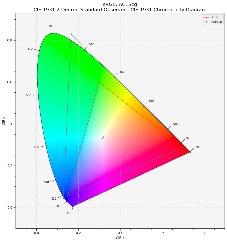
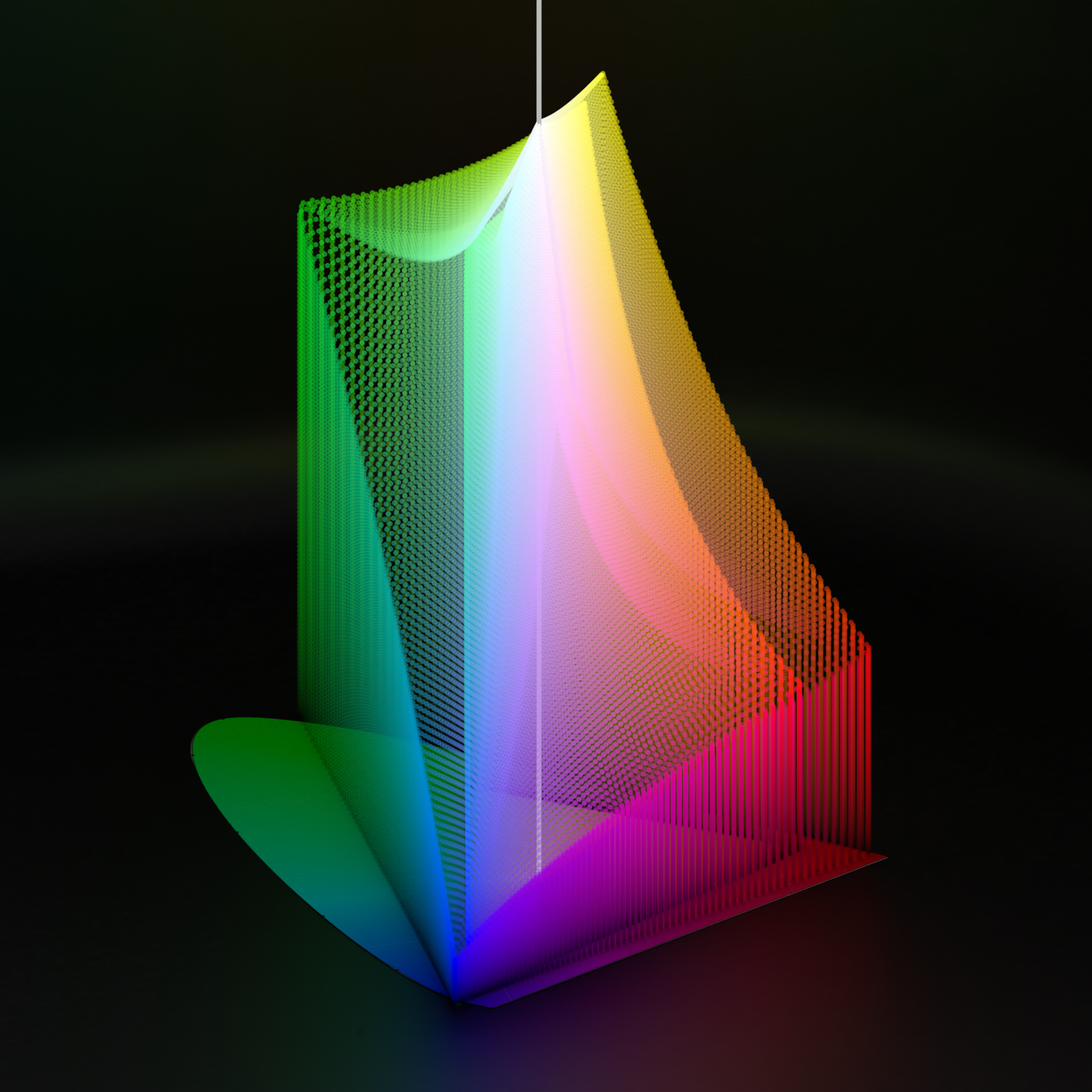
Most applications don’t let you freely choose a working color space — it comes baked into the software. Blender defaults to sRGB D65; DaVinci Resolve works in its own DaVinci YRGB space. OpenColorIO (OCIO) [5] exists to let different tools share one configurable pipeline instead of each hard-coding its own.
How the render space itself changes the image
This is the thesis’s central practical warning. Unlike a simple space-to-space conversion (which does preserve chromaticity), the color space a renderer computes in has a direct effect on the final colors, independent of anything that happens afterward.
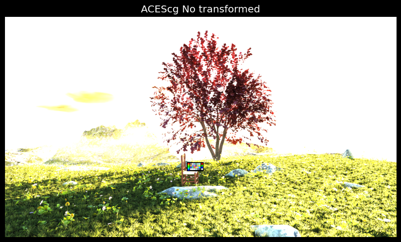
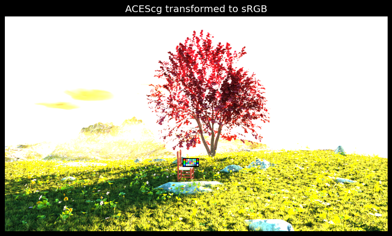
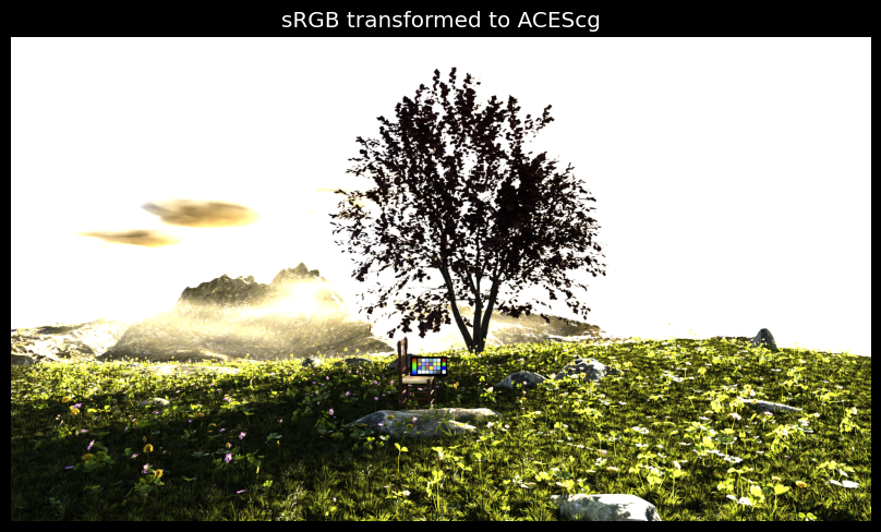
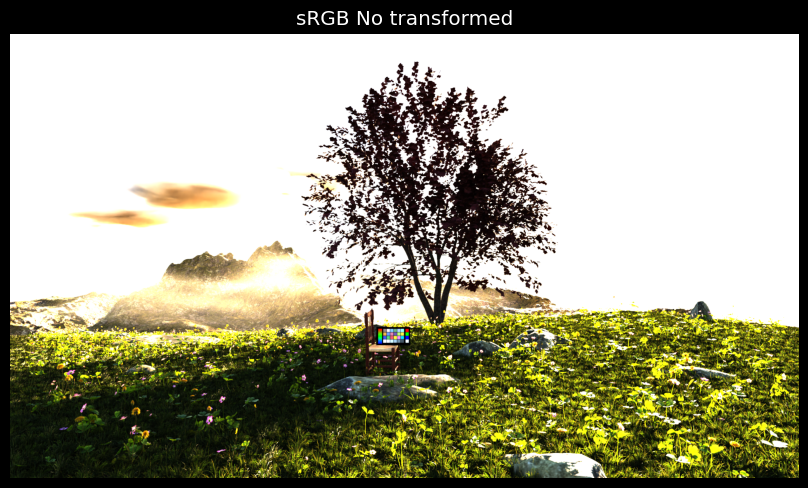
This happens because sRGB’s maximum green and ACEScg’s maximum green are not the same green — sRGB’s brightest green renders as a mid-green inside ACEScg — even though to a human viewer both still read as roughly “the same” green.
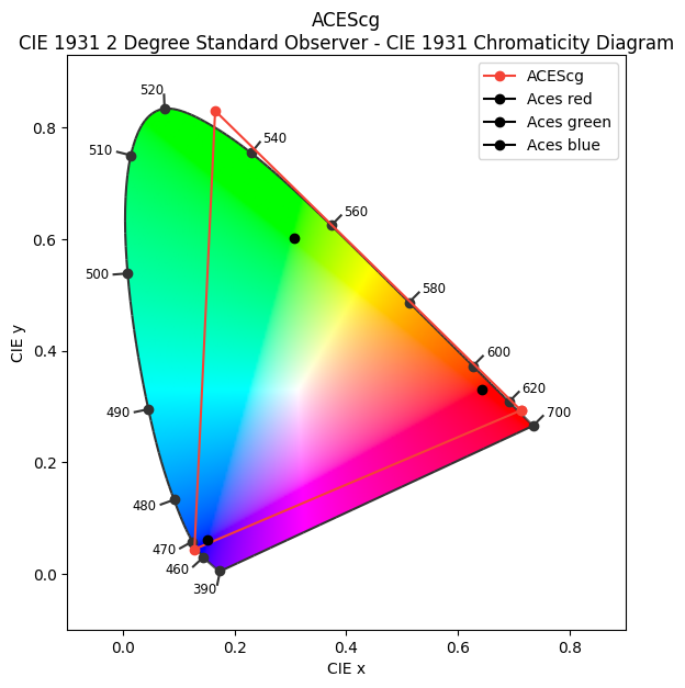
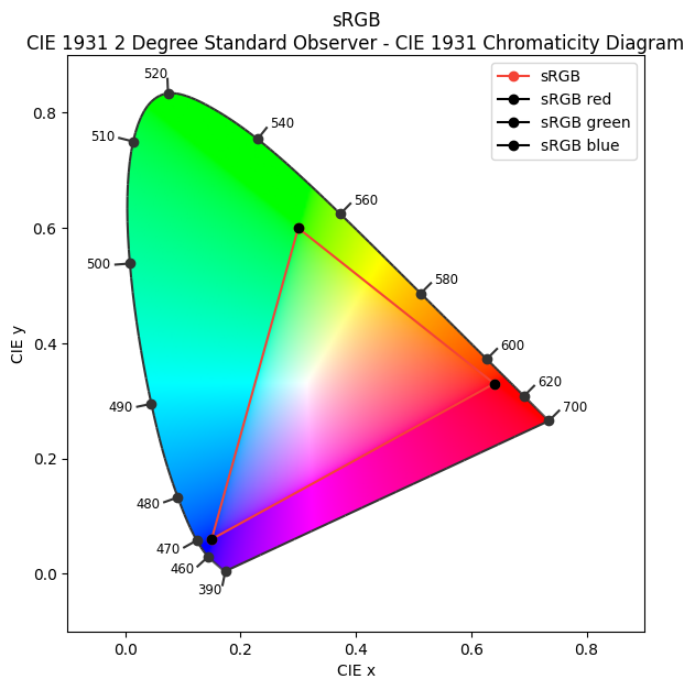
This is the core argument for treating ACES-like wide-gamut spaces as the working space for computation: calculations happen against colors closer to what human eyes can actually see, and only get compressed down to a narrower delivery space (sRGB, Rec.709…) at the very end.
Rolling off to white
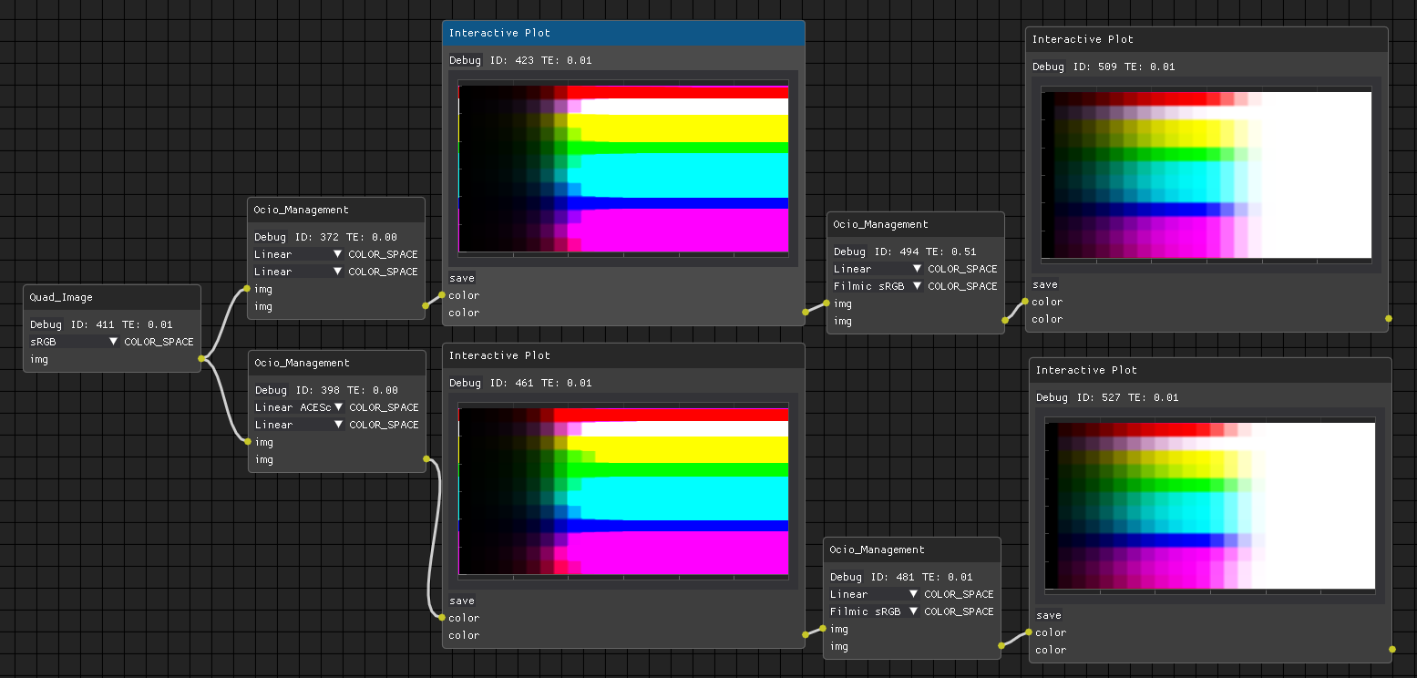
Interpreting channel luminosity also matters — via OETFs or LUTs. What happens if a linear ACEScg image and a linear sRGB image are both converted to sRGB (OETF included)?
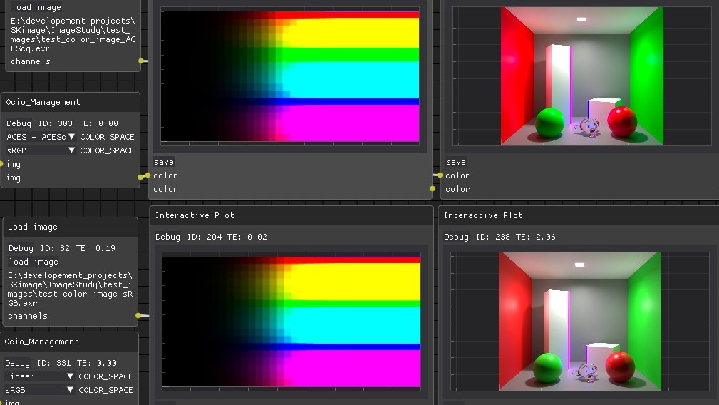
At very high intensities, colors freeze into pure primaries instead of rolling toward white — “the notorious six” [6: Ocio, display transforms and misconceptions; ; 2021]. The usual artistic fix is a more elaborate LUT, like the one Blender’s Filmic view transform uses, that bends those highlights back toward white instead of clipping into a saturated primary:
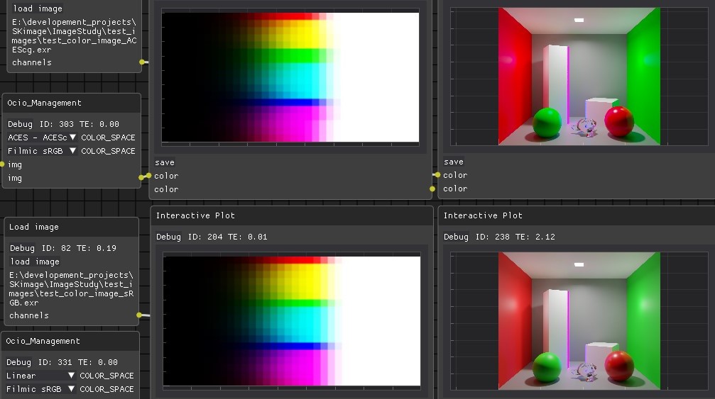
A “roll-off to white” like this is usually built from three stages: an allocation step that reshapes Scene-Referred light into Display-Referred space with a log-like curve (log2, Cineon…); a LUT or matrix that actually bends the highlights toward white (Blender ships this as a 3D cube LUT; AgX uses a fixed 3×3 matrix instead); and finally a standard OETF like sRGB to add the contrast a display needs.
The effect is visible directly on a rendered scene, not just a gradient — the same spheres, lit identically, render noticeably differently depending on whether the computation happened in sRGB or in ACEScg:
Converting between spaces
Moving data cleanly from one color space to another (assuming linear gamma) is a chain of well-defined matrix multiplications: from a working space like ACEScg into the ACES AP0 primaries, from AP0 into CIE XYZ, then — through a Profile Connection Space (PCS), almost always XYZ — a chromatic-adaptation step that re-maps the white point (Bradford being the most common adaptation matrix in practice), and finally from XYZ into the destination space, such as sRGB. Every well-behaved OCIO config implements exactly this chain; the practical takeaway is less about memorizing the matrices and more about knowing that this chain exists and trusting your tools’ bundled configs (Blender’s, Nuke’s, Resolve’s…) rather than re-deriving it by hand.
Dynamic range and bit depth are not the same thing
In a real scene, dynamic range is potentially infinite, and has to be compressed into a storable range before it can be processed at all. A RAW file stores 12–14 bits [7: Raw bit depth; ; 2017], which — in a perfect noiseless sensor — corresponds almost 1:1 to 12–14 EV of dynamic range; each extra bit doubles that range, and new bits are spent on the highlights.
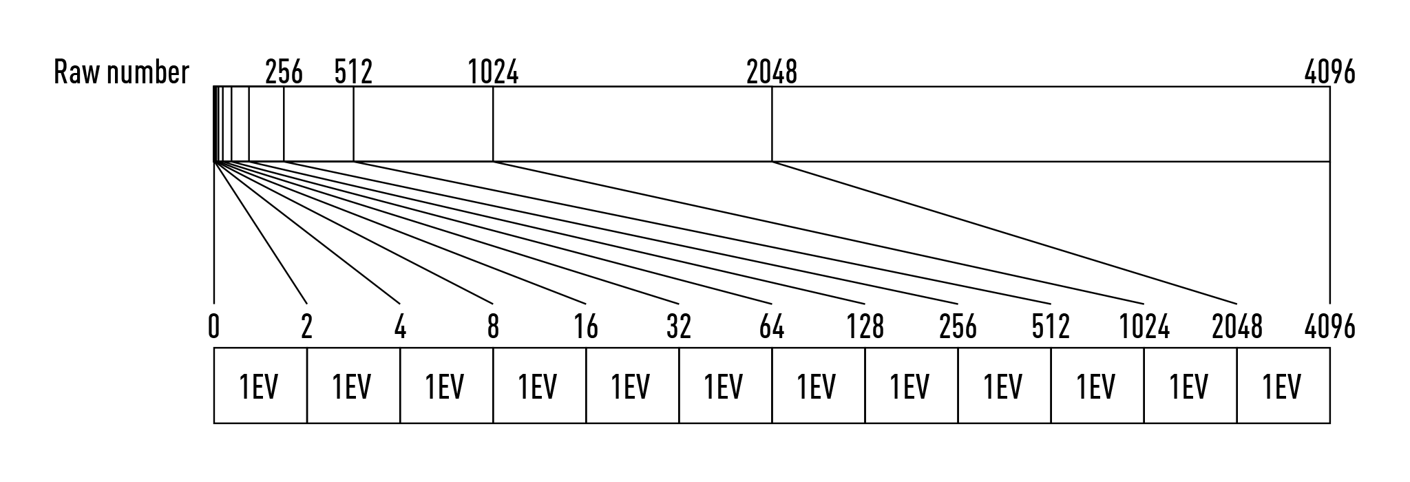
Bit depth and dynamic range are not the same thing, though it’s an easy conflation to make. A signal can be encoded with a tiny number of bits and still cover a huge range — 2 bits give 4 quantization steps, and a 0–1000 range can technically be encoded correctly (if uselessly) in those 4 steps. What more bits actually buy you is enough intermediate tones to avoid visible banding: too few gray levels between black and white, most noticeable in the shadows where human vision is most sensitive to small steps.
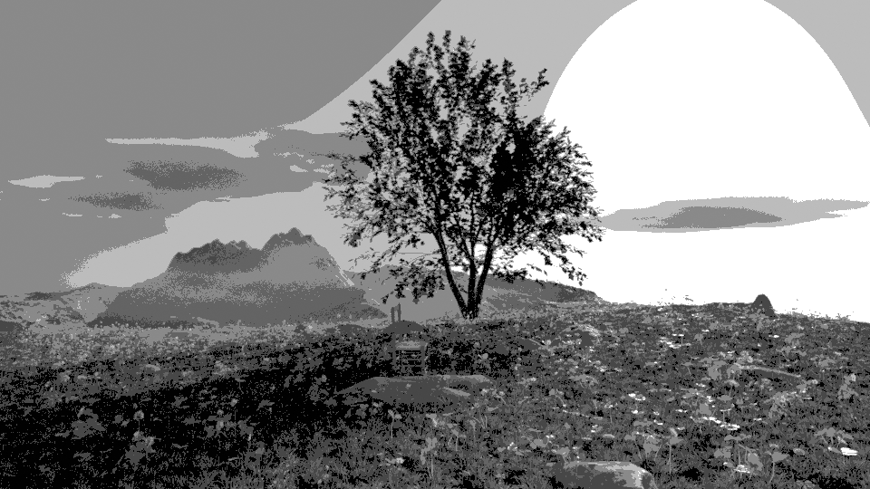
For CGI it’s more useful to describe a curve by its minimum encoded value, maximum encoded value, bit depth, and whether it uses a log-like reallocation than by “stops,” since the same 8-bit container can represent wildly different dynamic ranges depending on which curve is applied:
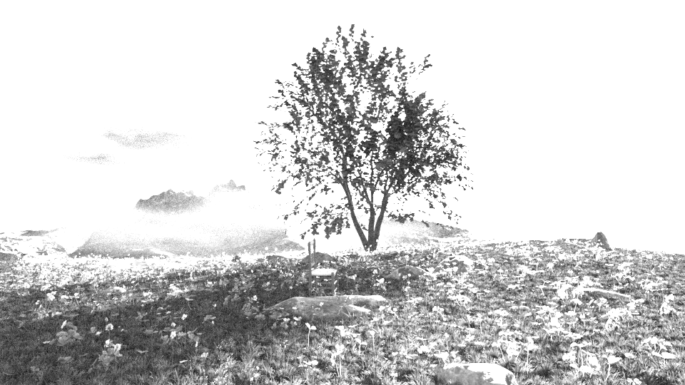
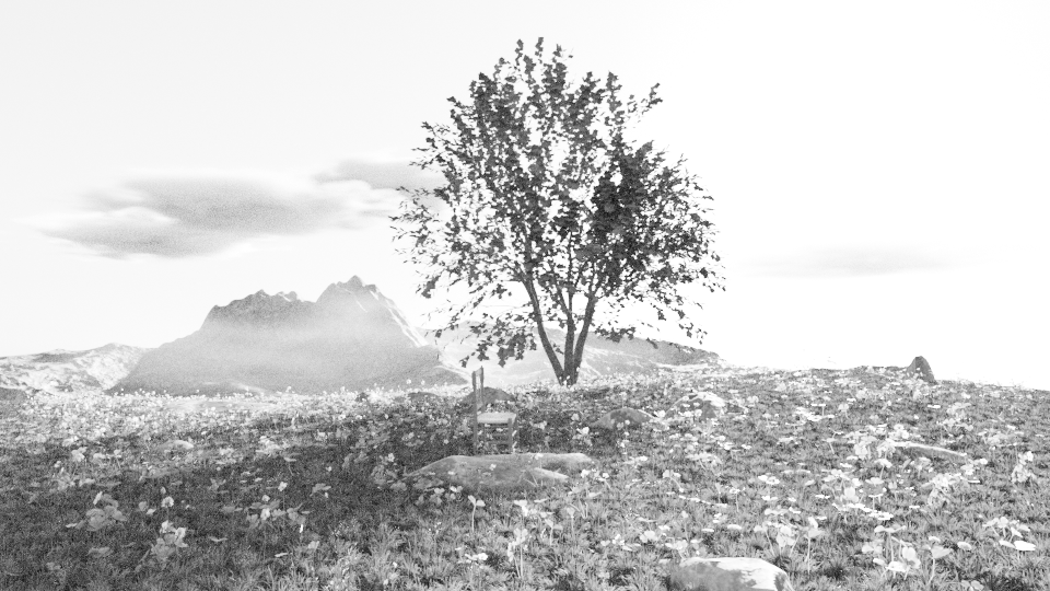
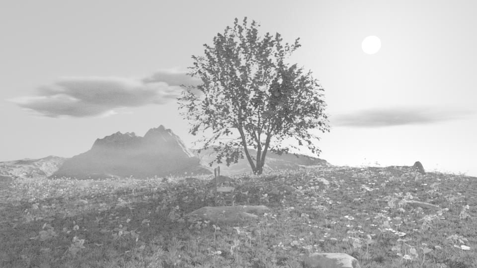
Formats that can only store values between 0 and 1, like PNG, get no benefit from extra bit depth for highlights — every extra bit just adds resolution to the shadows, since the highlights are already clipped at 1.0 regardless of bit depth. Push a wide dynamic range through too few bits and banding artifacts appear exactly where the display curve compresses the most:



Even so, the 0–1 range by itself carries a lot of usable information — a well-exposed sRGB image still reads fine several stops under its nominal exposure:
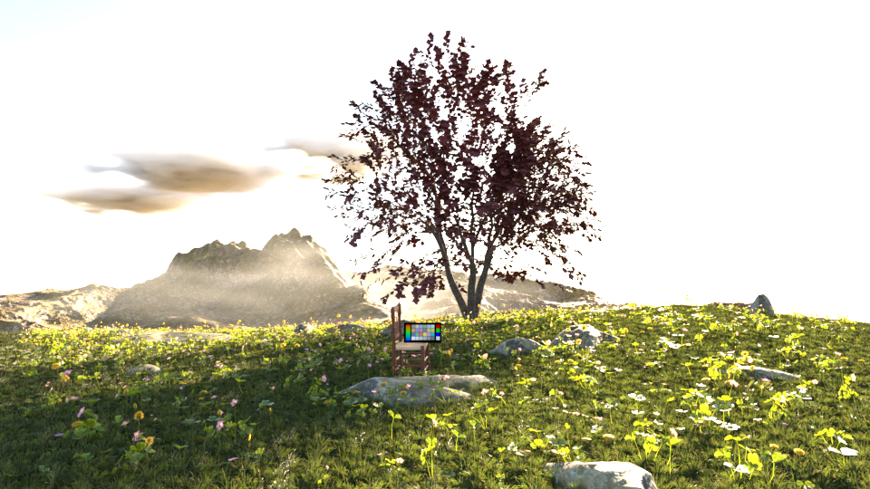
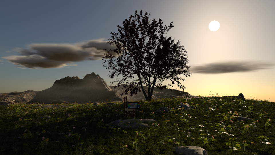
For images meant for further manipulation — compositing, CGI integration — you generally need more headroom than a straight 0–1 image gives you, and there are three ways to get it: more bit depth (best quality and versatility, at a real disk-space cost); a specialized, non-pretty log-like OETF that trades highlight resolution for extra shadow detail; or a format built to combine both, like DPX, which supports selectable bit depth and an optional CINEON log curve in the same container.
Transfer functions, OETFs and LUTs
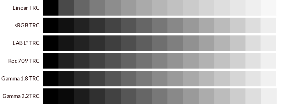
An OETF (Opto-Electric Transfer Function) reshapes light so shadows get better resolution (avoiding banding) and highlights compress into the 0–1 range (tone mapping). OETFs meant for final display are usually tuned to look good at low bit depth — expressed as a “perceptually linear” gradient, which is not the same as a physically linear one: a purely linear gradient’s darkest step reads as a huge jump from pure black, while its brightest steps are barely distinguishable from each other.
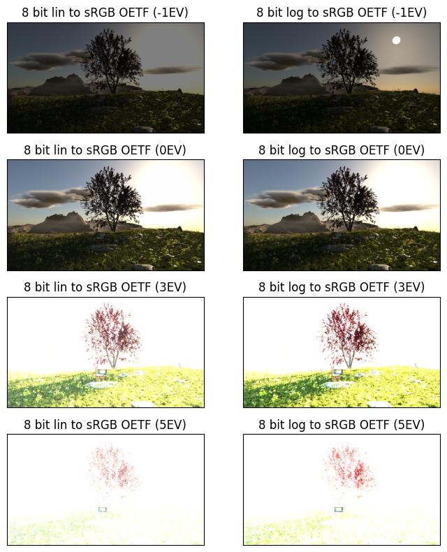
Other OETFs exist purely to preserve information for later use rather than to look pleasant — the log curves. Recovering a scene’s real linear values later is dramatically easier from a log-encoded image than from a straight Display-Referred one:
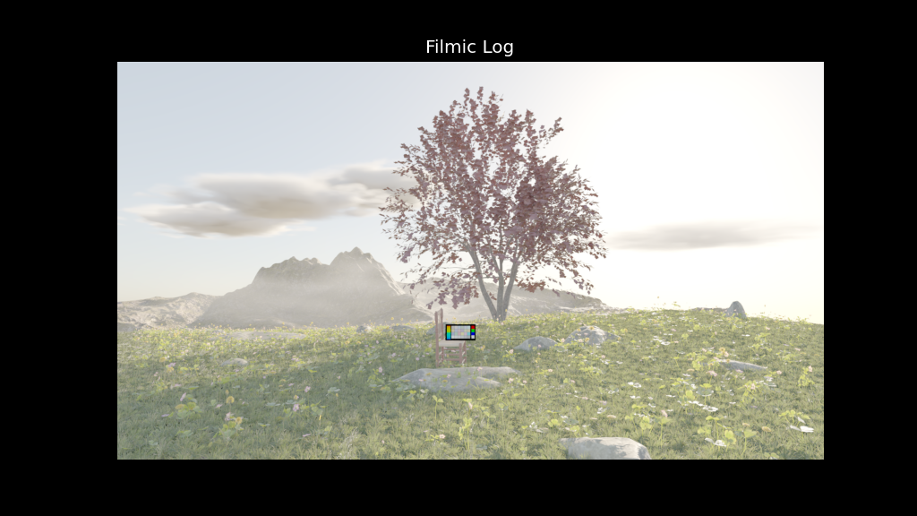
A handful of well-known log curves, each trading shadow/highlight allocation slightly differently — Filmic Log, Log2, LogC (ARRI), S-Log2 (Sony):
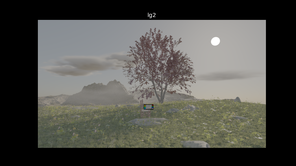
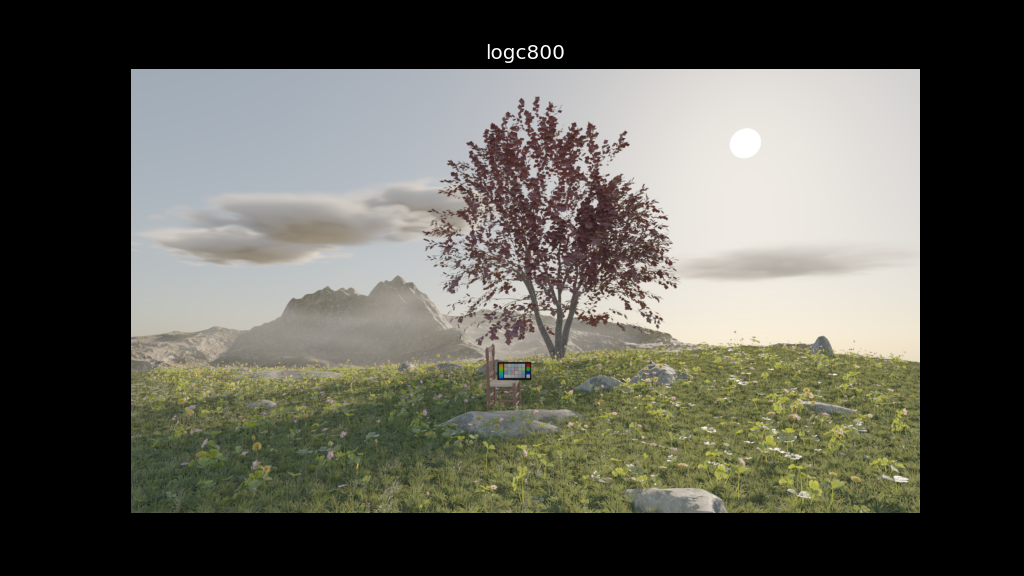
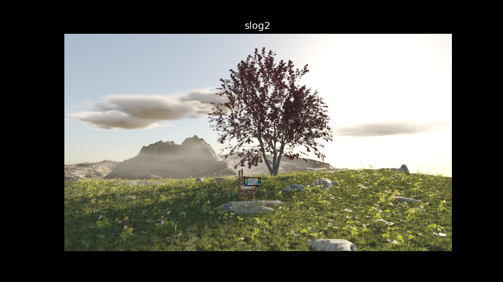
To be precise about terms: OETFs are the mathematical functions applied to reshape values between linear and non-linear color — this includes gammas, LUTs, and Look Modification Transforms. The sRGB OETF, for instance, is a piecewise function rather than a single clean exponent:
LUTs, meanwhile, are just lookup tables that map inputs to outputs — the mechanism most complex OETFs and creative looks are actually stored as, since curves like sRGB and rec.709 rarely get re-derived from formula every time a program needs them. A 1D LUT handles the transfer curve; a 3D .cube/.spi3d LUT can additionally handle full-color creative looks by accounting for every possible input combination at once.
Open Color IO
OCIO [5] is a complete, open-source color-management solution built for film and VFX production. It gives every compatible application a consistent user experience while allowing very sophisticated configuration underneath, and it’s ACES-aware and LUT-format-agnostic.
An OCIO config is a single config.ocio file: it declares a Profile Connection Space, named color spaces with to_reference/from_reference transforms (LUTs, matrices, 3D cubes), a set of displays and views, and roles mapping generic names like scene_linear to a concrete space. Nuke, Blender and Resolve each ship their own config tuned to their own render space and LUTs — using one of these proven configs, rather than writing your own from scratch, avoids most conversion mistakes.
Blender’s stock config is a good worked example of a “roll-off to white”: its Filmic Log color space allocates Scene-Referred light onto a log2 curve spanning roughly -12.47 to +12.53 stops, runs it through a desaturating 3D LUT (filmic_desat65cube.spi3d), and only then does Filmic sRGB chain that log space into a final 1D LUT and display OETF.
Image formats
The industry generally settles on high-bit-depth formats (16–32 bit) for CGI and VFX work — 16-bit PNG, 16–32-bit EXR, 16-bit TIFF — and they differ mainly in what the stored values actually represent:
| Format | Bit depth | Data type | Color space |
|---|---|---|---|
| BMP | 8 | uint | OETF |
| PNG | 8, 16 | uint | OETF |
| JPEG [8: Performance Comparison of Jpeg, Jpeg XT, Jpeg LS, Jpeg 2000, Jpeg XR, HEVC, EVC and VVC for Images; ; 2021] | 8 | uint | OETF |
| JPEG 2000 [8: Performance Comparison of Jpeg, Jpeg XT, Jpeg LS, Jpeg 2000, Jpeg XR, HEVC, EVC and VVC for Images; ; 2021] | 8, 12, 16 | uint | OETF |
| Targa [9: Truevision TGA: FILE FORMAT SPECIFICATION VERSION 2.0; ; 1991] | 8, 15, 16, 24, 32 | uint | OETF |
| Cineon [10: Understanding Cineon; ; 2001] | 8, 10, 12, 16 | uint | linear (log-encoded) |
| DPX [11: ST 268:2003 - SMPTE Standard - For File Format for Digital Moving-Picture Exchange (DPX), Version 2.0; 2003] | 8, 10, 12, 16 | uint | linear (log-encoded) |
| OpenEXR [12] | 16, 32 | float / half-float | linear |
| Radiance HDR [13: RGBD Archives; ; 2013] | 8 | uint (RGBE) | linear |
| TIFF [14: TIFF; ; 1992] | 8, 16 | uint | OETF |
| WebP [15] | 8 | uint | OETF |
OpenEXR is the default choice for CGI production because of its float precision and arbitrary multi-channel layout (color, normals, cryptomatte IDs, all in one file). Its half-float encoding stores more precision near zero than near its maximum [16: Half-precision floating-point, visualized; ; 2021], mirroring how humans perceive brightness — which is exactly why applying a display transfer function before saving to EXR (instead of after) throws away the format’s main advantage. That flexibility has a real disk-space cost, though: a 150-frame 1080p sequence ranges from tens of megabytes (WebP, JPEG) up to several gigabytes, depending on the EXR compression scheme chosen — the “just use EXR for everything” instinct needs to be weighed against actual project needs.
Display technology
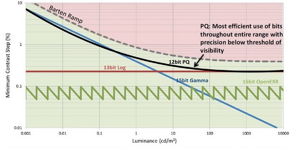
Consumer HDR technology (Dolby Vision, HDR10, HDR10+) typically works at 10–12 bit depth with Rec.2020 primaries and a PQ (Perceptual Quantizer) transfer function [17: 2018 Update on High Dynamic Range Television; ; 2018], designed so a fixed number of code values maps to visually even steps of absolute brightness — unlike SDR curves, which are relative to a reference white. HDR10 targets 10 bits as enough to avoid visible banding; Dolby Vision uses 12. Since PQ is incompatible with the Rec.709 curve SDR displays use, HDR and SDR masters are usually graded as two separate deliverables from the same source.
A proposed open color pipeline
Building on all of the above, the thesis proposes a small, coherent color-management scheme aimed at VFX/CGI generalists: Rec.2020 as the working (rendering) space — its gamut sits close to a full spectral render [18: Anders Langlands; ] while staying inside the CIE 1931 horseshoe (unlike ACEScg, which extends slightly beyond it) — paired with a Display Rendering Transform based on Jed Smith’s OpenDRT [19: Jedypod/open-display-transform: Open display transform is a collection of tools and experiments for rendering wide-gamut scene-linear data into an image for an SDR or HDR display device.; ]: gamut mapping from the render space to the output space, a tone scale, and chroma-preserving compression toward white in the highlights.
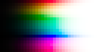
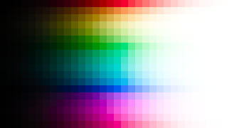
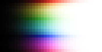
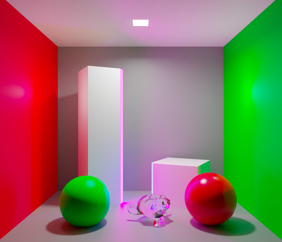
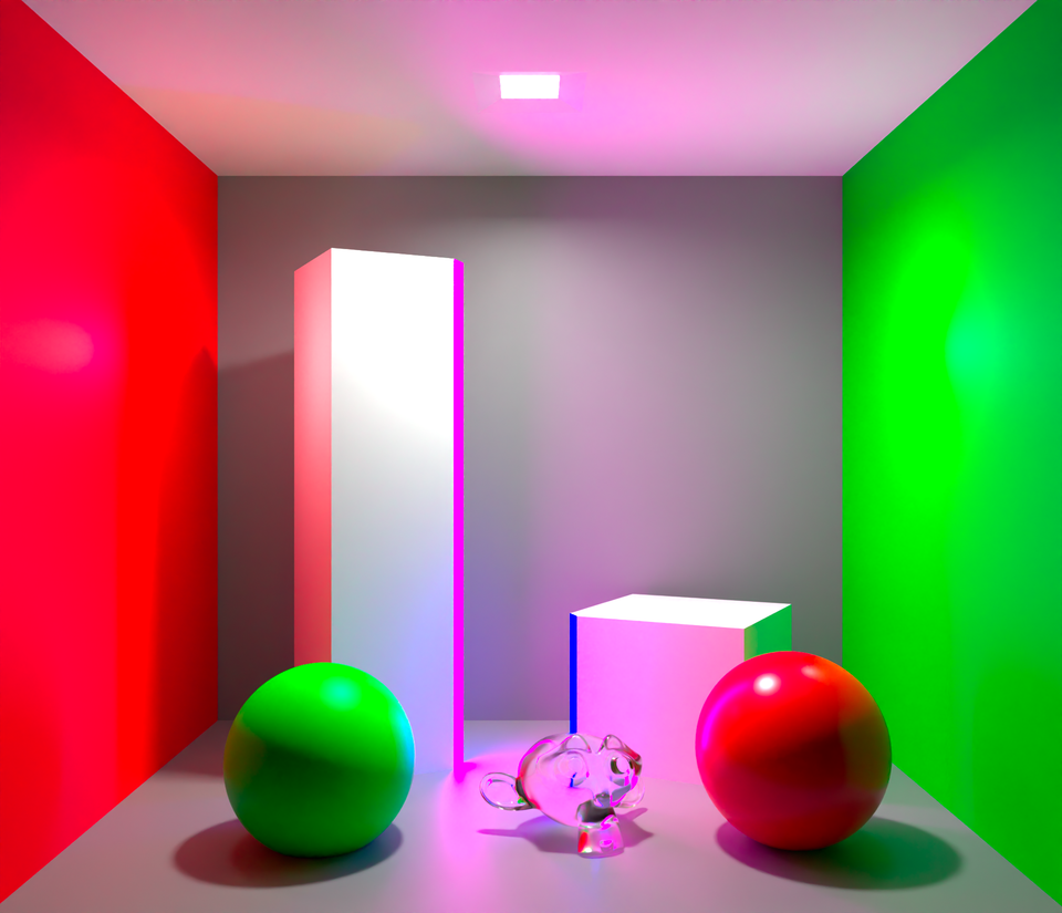
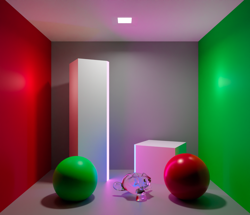
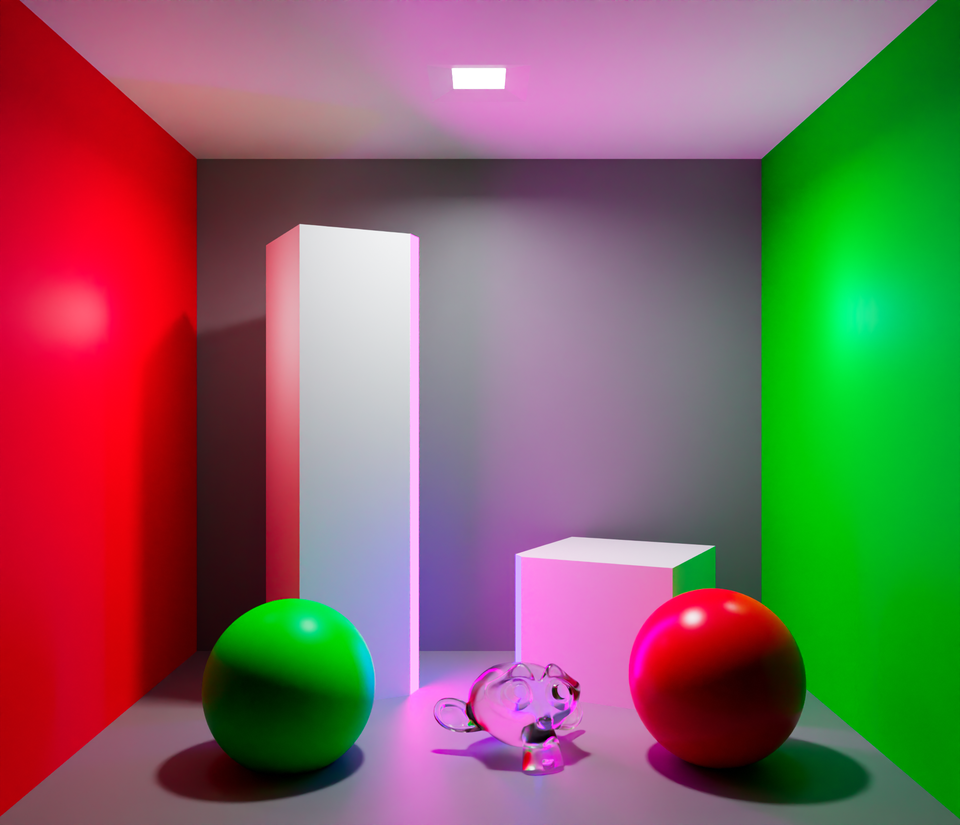
That pipeline became an actual OCIO config and a set of 3D LUTs, generated with a small Python routine that samples a 65³ cube, converts each sample from Display-Referred back to Scene-Referred, runs it through the DRT, and re-encodes the resulting table — the same kind of workflow Chris Brejon discusses [6: Ocio, display transforms and misconceptions; ; 2021] for OCIO display transforms. On a real test scene, the OpenDRT transform holds onto the best reflections and emissive-material highlights, while the other transforms give a subjectively different “sense of luminosity”:
Study Image: a node-based tool for studying color
The concrete software contribution is Study Image, a lightweight, node-based application written entirely in Python (dearpygui), built to fill a specific gap: none of the mainstream tools are both fast to open and simple to extend. Blender doesn’t load RAW files; Nuke opens raw images and does node compositing well but has a steep learning curve for a generalist; Photoshop and Lightroom are the usual stopgap for RAW-to-standard-format conversion.
Design goals were explicit: lightweight and fast (no heavier than needed just to inspect images and color spaces); visual and step-by-step (every operation inspectable, not a black box); OCIO-native (color management goes through real OCIO configs, portable to Blender, Nuke or Resolve); and simple, hackable code (a new node is a plain Python function plus a small class — no plugin SDK to learn).
How the node graph executes
Node-based applications typically execute asynchronously, working backward from a single output node and calling only the upstream nodes actually needed:
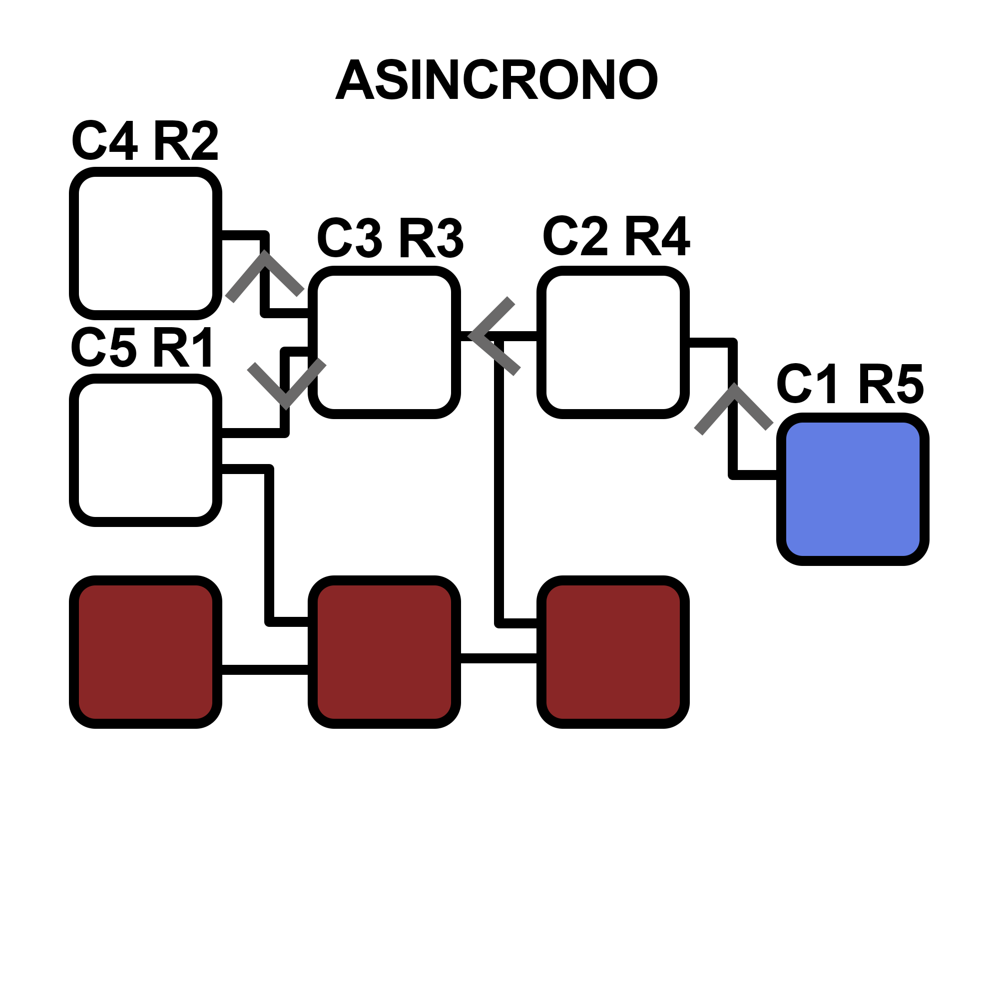
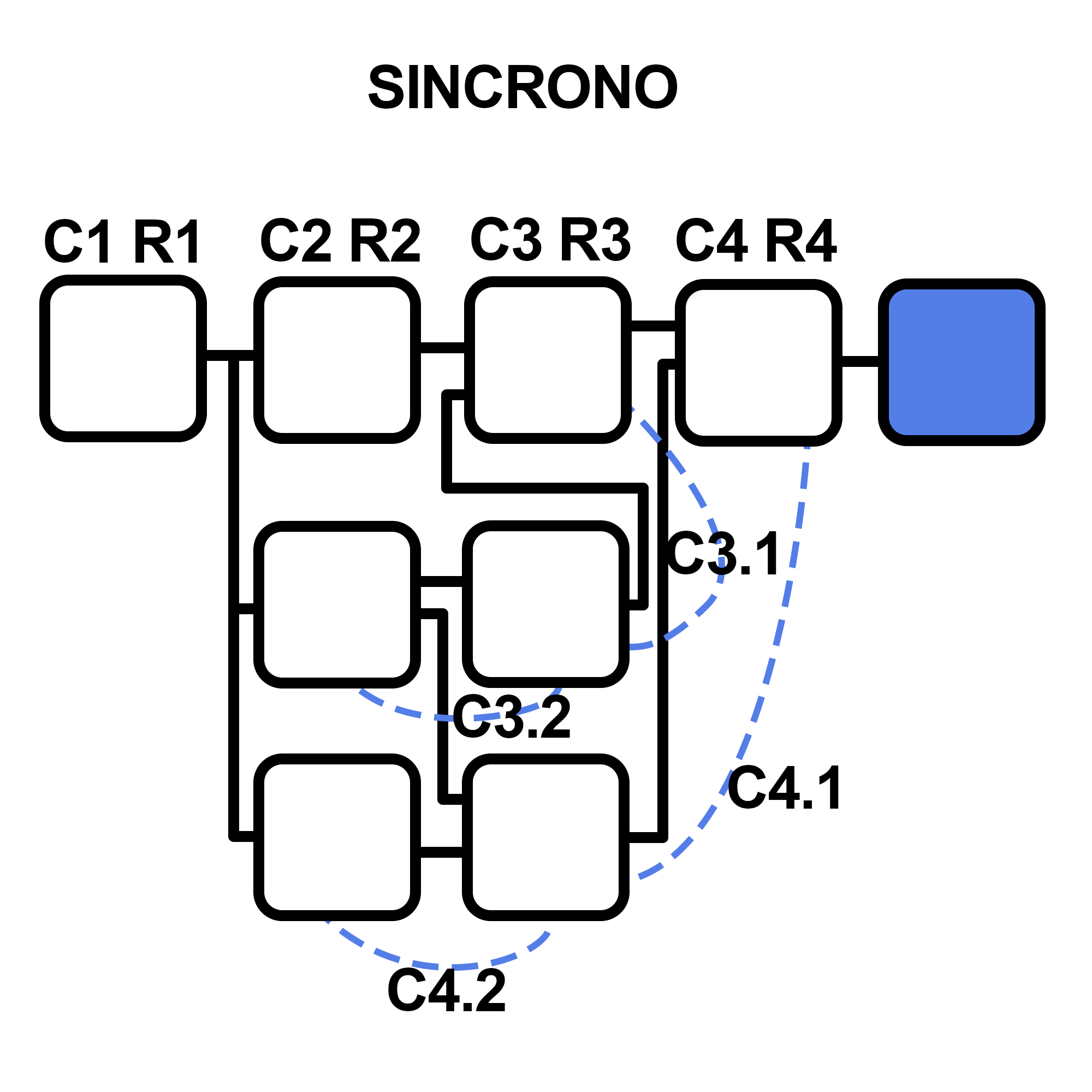
Study Image deliberately does the opposite: it can have multiple independent output nodes rather than one single sink, which complicates a purely output-driven executor. Instead, it runs synchronously, forward from any modified node — every node caches its own output and a record of “already executed” nodes; changing a node clears that record for itself and everything downstream, and only that subgraph re-runs:
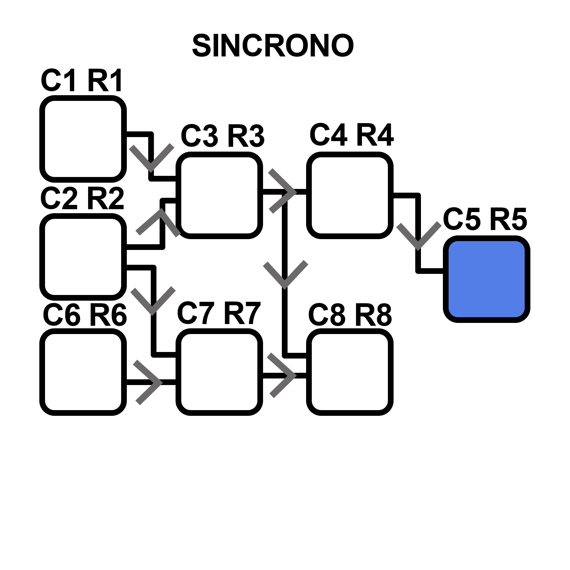
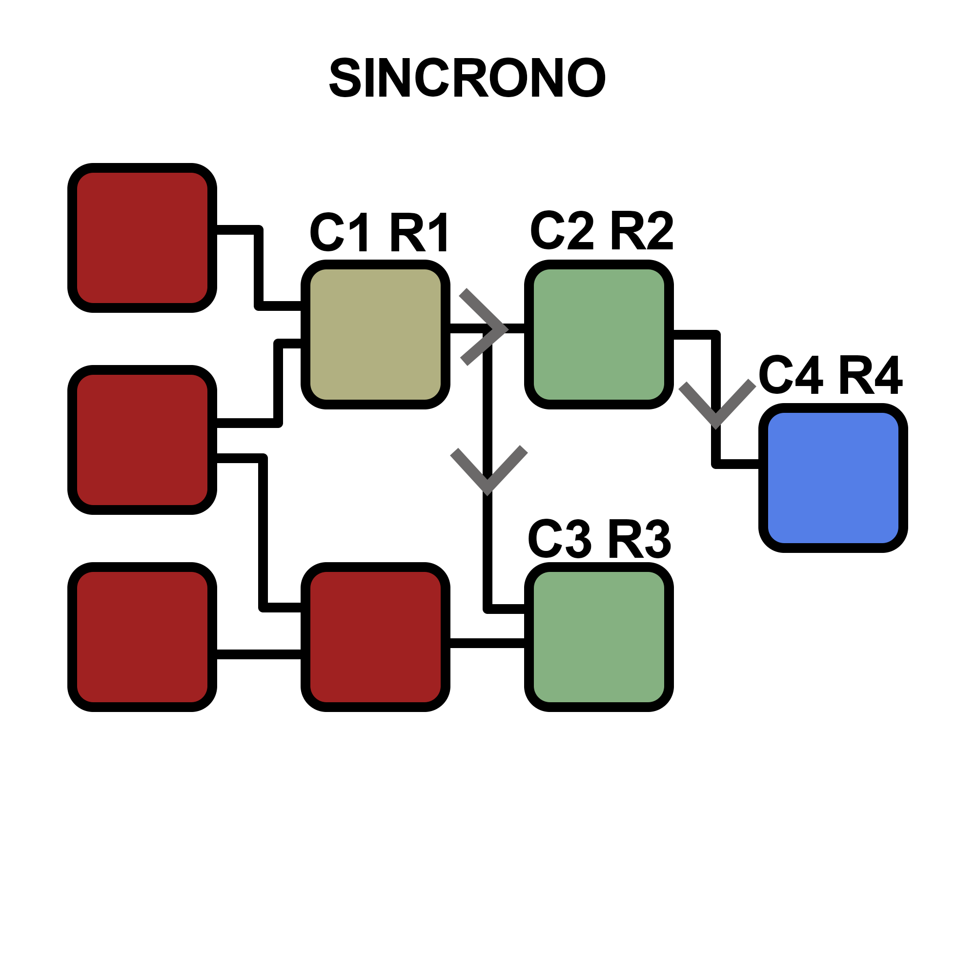
The one wrinkle this design has to handle explicitly: a node that depends on other nodes which haven’t executed yet must wait its turn rather than running with stale or missing inputs.
Building a node
Every node follows the same three-part layout — a header (name, plus a shared debug line with execution time and node ID), a static area for custom widgets the user adds freely, and colored pins for inputs/outputs:
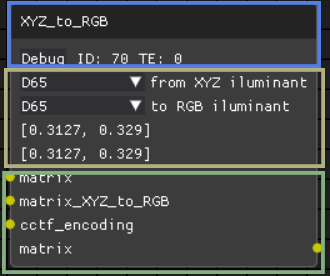
A minimal new node is just a function plus a small subclass declaring its title, its input/output pin names, and any custom widgets to place in the static area — no plugin SDK, just plain Python:
def exposition(val1, val2, *argss):
    return [val1 ** val2]

class Exposition(NodeV2):
    Title = "Exposition"
    def __init__(self):
        inp_list = {"val": {"slider": {"width": 120}},
                     "exp": {"value": {"width": 120, "format": '%.8f'}}}
        out_list = ["val"]
        super().__init__(exposition, inp_list, out_list, self.Title)
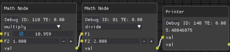
Input pins can carry small interactive widgets (a slider, a numeric field) that disappear automatically the moment another node gets connected to that pin:
What it does
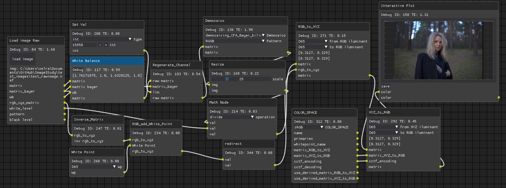
- RAW image processing — the full pipeline described above, exposed as inspectable nodes.
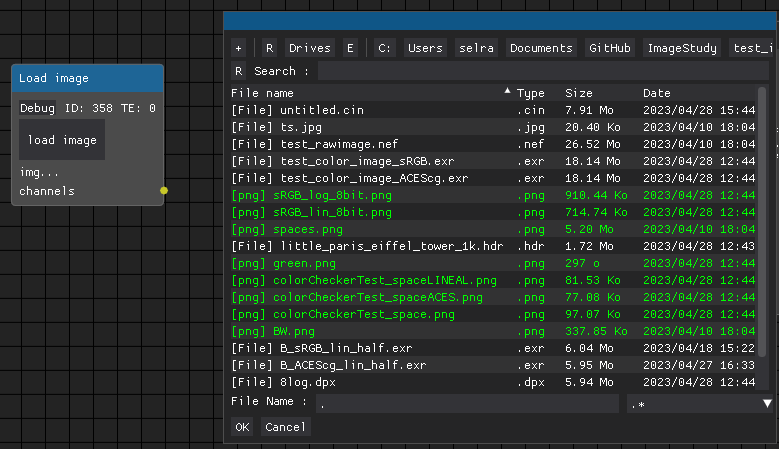
- Loading a wide range of formats — JPG, PNG, HDR, TIFF, EXR, DPX and more.
- Full OCIO-based color management and transforms.
- Image viewing and saving.
- Tools for catching color-management artifacts before they reach a shot — false-color exposure checks, side-by-side transform comparisons.
- A simple API for adding new nodes with custom, user-defined functions.
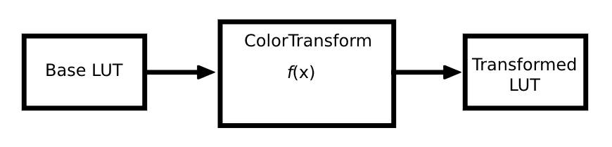
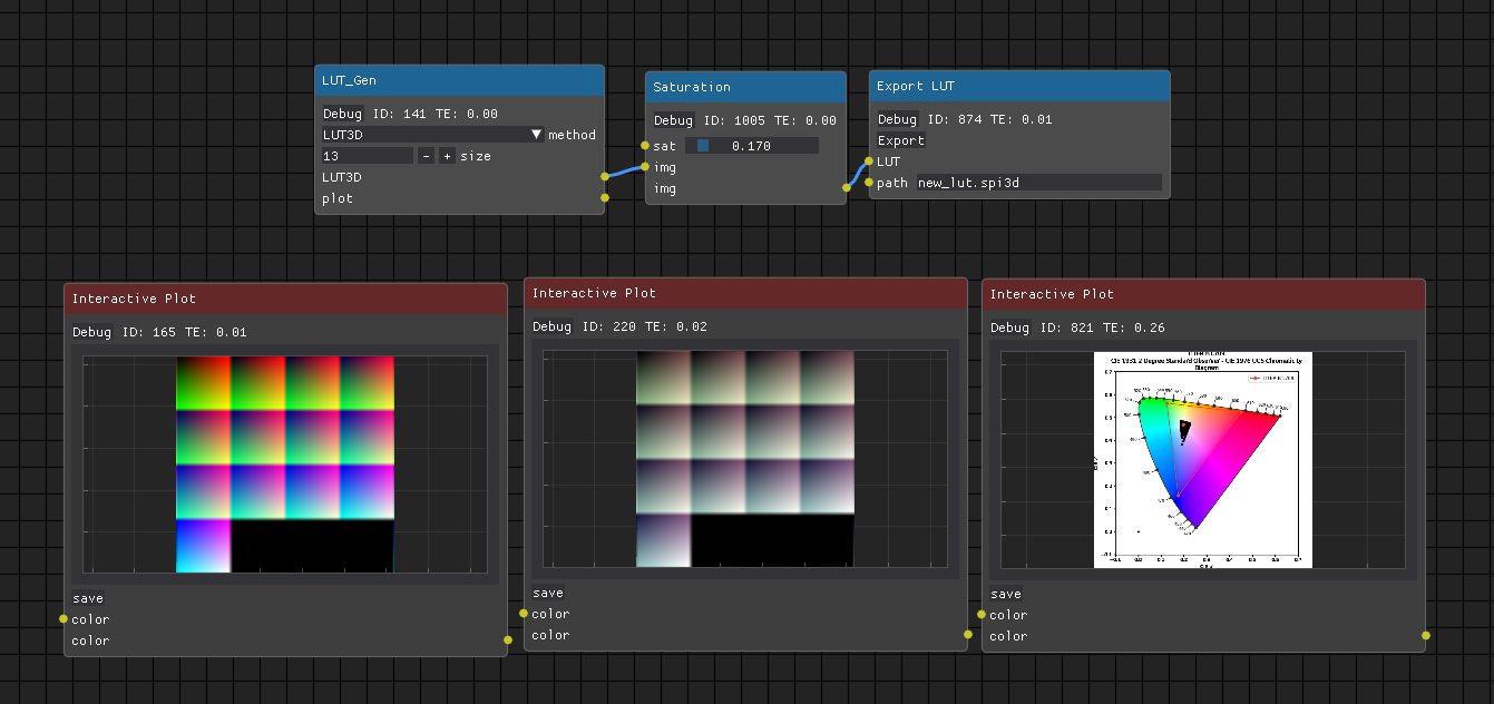
A worked example: building a LUT from scratch
A full color-pipeline workflow — from a loaded image through a color transform to a saved LUT — collapses into a handful of connected nodes:
Catching problems before they reach a shot
Study Image includes a False Color exposure tool that segments an image’s luminance into bands, making it easy to spot clipped highlights or crushed shadows at a glance — this is the screenshot used as this post’s header image:
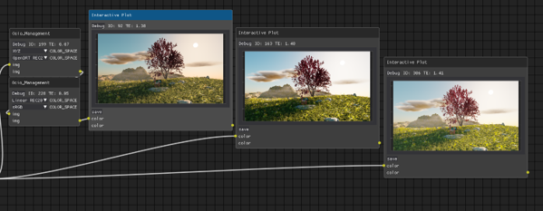
It also makes comparing color transforms fast — side by side, instead of one at a time:
The full source is on GitHub: Study-Image-Code.
A Blender color-management addon
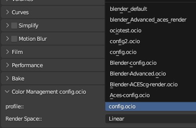
Blender’s built-in color management is intentionally minimal — one OCIO config, one input transform per image, one output space. As a companion to the thesis, I built an addon that lets you switch between custom OCIO configs stored anywhere in your Blender config (not just the bundled one), adds built-in support for ACEScg/ACES, AgX base and looks, Cineon Log, and in-program switching of the render-time working space (sRGB vs. ACEScg primaries), and ships an expanded internal config (blender_Advanced) adding AgX and Filmic looks, the experimental OpenDRT transform from this thesis, ACES output transforms, a reorganized [sRGB, XYZ, Utils] display layout, and naming consistent between Blender’s and ACES’ own conventions.
Conclusion
Unifying camera-captured and computer-generated imagery under one color pipeline is not a solved problem — it depends on the specific cameras, renderers, and delivery targets involved. But a two-stage separation, computing in a space that covers the visible spectrum and applying a single, well-understood Display Rendering Transform on the way out, gives CGI the same starting point as photographed material: comparable storage requirements, the same dynamic-range characteristics, and identical behavior under color grading — turning what is usually a case-by-case integration headache into a standard, repeatable process.
Bibliography
- , "The Principles of Color Management", Springer Berlin Heidelberg, 2009, DOI | URL.
- , "Light Objects", Light Objects - Blender Manual, 2023, URL.
- , "Artificial Lighting System for Plant Growth and Development: Chronological Advancement, Working Principles, and Comparative Assessment", Light Emitting Diodes for Agriculture: Smart Lighting, pp. 1-25, 2017, DOI.
- , "Colorimetry - 4th Edition", CIE Central Bureau, 2018.
- , "Untitled", Unknown Year, URL.
- , "Ocio, display transforms and misconceptions", ocio display transforms and misconceptions, 2021, URL.
- , "Raw bit depth", Richard Butler, 2017, URL.
- , "Performance Comparison of Jpeg, Jpeg XT, Jpeg LS, Jpeg 2000, Jpeg XR, HEVC, EVC and VVC for Images", 2021, DOI.
- , "Truevision TGA: FILE FORMAT SPECIFICATION VERSION 2.0", Truevision, Inc., 1991, URL.
- , "Understanding Cineon", 2001, URL.
- "ST 268:2003 - SMPTE Standard - For File Format for Digital Moving-Picture Exchange (DPX), Version 2.0", ST 268:2003, pp. 1-17, 2003, DOI.
- , "Untitled", Technical Introduction to OpenEXR, Unknown Year, URL.
- , "RGBD Archives", Light is beautiful, 2013, URL.
- , "TIFF", 1992, URL.
- , "Untitled", DotWhat.net, Unknown Year, URL.
- , "Half-precision floating-point, visualized", Observable, 2021, URL.
- , "2018 Update on High Dynamic Range Television", SMPTE Motion Imaging Journal, vol. 127, pp. 91-93, 2018, DOI.
- , "Anders Langlands", Render Color Spaces, Unknown Year, URL.
- , "Jedypod/open-display-transform: Open display transform is a collection of tools and experiments for rendering wide-gamut scene-linear data into an image for an SDR or HDR display device.", GitHub, Unknown Year, URL.